Quantcast
Channel: Daniel Berman is Product Evangelist at Logz.io
Viewing all 198 articles
Browse latest View live

How to Monitor AWS EC2 with Metricbeat, the ELK Stack and Logz.io

$
0
0

Amazon EC2 is the cornerstone for any Amazon-based cloud deployment. Enabling you to provision and scale compute resources with different memory, CPU, networking and storage capacity in multiple regions all around the world, EC2 is by far Amazon’s most popular and widely used service.

Monitoring EC2 is crucial for making sure your instances are available and performing as expected. Metrics such as CPU utilization, disk I/O, and network utilization, for example, should be closely tracked to establish a baseline and identify when there is a performance problem.

Conveniently, these monitoring metrics, together with other metric types, are automatically shipped to Amazon CloudWatch for analysis. While it is possible to use the AWS CLI, API or event the CloudWatch Console to view these metrics, for deeper analysis and more effective monitoring, a more robust monitoring solution is required.

In this article, I’d like to show how to ship EC2 metrics into the ELK Stack and Logz.io. The method I’m going to use is a new AWS module made available in Metricbeat version 7 (beta). While still under development, and as shown below, this module provides an extremely simple way for centrally collecting performance metrics from all your EC2 instances.

Prerequisites

I assume you already have either your own ELK Stack deployed or a Logz.io account. For more information on installing the ELK Stack, check out our ELK guide. To use the Logz.io community edition, click here.

Step 1: Creating an IAM policy

First, you need to create an IAM policy for pulling metrics from CloudWatch and listing EC2 instances. Once created, we will attach this policy to the IAM user we are using.

In the IAM Console, go to Policies, hit the Create policy button, and use the visual editor to add the following permissions to the policy:

  • ec2:DescribeRegions
  • ec2:DescribeInstances
  • cloudwatch:GetMetricData

The resulting JSON for the policy should look like this:

{
    "Version": "2012-10-17",
    "Statement": [
        {
            "Sid": "VisualEditor0",
            "Effect": "Allow",
            "Action": [
                "ec2:DescribeInstances",
                "cloudwatch:GetMetricData",
                "ec2:DescribeRegions"
            ],
            "Resource": "*"
        }
    ]
}

Once saved, attach the policy to your IAM user.

Step 2: Installing Metricbeat

Metricbeat can be downloaded and installed using a variety of different methods, but I will be using Apt to install it from Elastic’s repositories.

First, you need to add Elastic’s signing key so that the downloaded package can be verified (skip this step if you’ve already installed packages from Elastic):

wget -qO - https://artifacts.elastic.co/GPG-KEY-elasticsearch | 
sudo apt-key add -

The next step is to add the repository definition to your system. Please note that I’m using the 7.0 beta repository since the AWS module is bundled with this version only for now:

echo "deb https://artifacts.elastic.co/packages/7.x-prerelease/apt stable 
main" | sudo tee -a /etc/apt/sources.list.d/elastic-7.x-prerelease.list

All that’s left to do is to update your repositories and install Metricbeat:

sudo apt-get update && sudo apt-get install metricbeat

Step 3: Configuring Metricbeat

Before we run Metricbeat, there are a few configurations we need to apply.

First, we need to disable the system module that is enabled by default. Otherwise, we will be seeing system metrics in Kibana collected from our host. This is not mandatory but is recommended if you want to keep a cleaner Kibana workspace.

sudo metricbeat modules disable system

Verify with:

ls /etc/metricbeat/module.d

envoyproxy.yml.disabled     kvm.yml.disabled         postgresql.yml.disabled
aerospike.yml.disabled      etcd.yml.disabled        logstash.yml.disabled   prometheus.yml.disabled
apache.yml.disabled         golang.yml.disabled      memcached.yml.disabled  rabbitmq.yml.disabled
aws.yml.disabled            graphite.yml.disabled    mongodb.yml.disabled    redis.yml.disabled
ceph.yml.disabled           haproxy.yml.disabled     mssql.yml.disabled      system.yml.disabled
couchbase.yml.disabled      http.yml.disabled        munin.yml.disabled      traefik.yml.disabled
couchdb.yml.disabled        jolokia.yml.disabled     mysql.yml.disabled      uwsgi.yml.disabled
docker.yml.disabled         kafka.yml.disabled       nats.yml.disabled       vsphere.yml.disabled
dropwizard.yml.disabled     kibana.yml.disabled      nginx.yml.disabled      windows.yml.disabled
elasticsearch.yml.disabled  kubernetes.yml.disabled  php_fpm.yml.disabled    zookeeper.yml.disabled

The next step is to configure the AWS module.

sudo vim /etc/metricbeat/module.d/aws.yml.disabled

Add your AWS IAM user credentials to the module configuration as follows:

- module: aws
  period: 300s
  metricsets:
    - "ec2"
  access_key_id: 'YourAWSAccessKey'
  secret_access_key: 'YourAWSSecretAccessKey'
  default_region: 'us-east-1'

In this example, we’re defining the user credentials directly but you can also refer to them as env variables if you have defined as such. There is also an option to use temporary credentials, and in that case you will need to add a line for the session token. Read more about these options in the documentation for the module.

The period setting defines the interval at which metrics are pulled from CloudWatch.

To enable the module, use:

sudo metricbeat modules enable aws

Shipping to ELK

To ship the EC2 metrics to your ELK Stack, simply start Metricbeat (the default Metricbeat configuration has a locally Elasticsearch instance defined as the output so if you’re shipping to a remote Elasticsearch cluster, be sure to tweak the output section before starting Metricbeat):

sudo service metricbeat start

Within a few seconds, you should see a new metricbeat-* index created in Elasticsearch:

health status index                                    uuid                   pri rep docs.count docs.deleted store.size pri.store.size
green  open   .kibana_1                                kzb_TxvjRqyhtwY8Qxq43A   1   0        490            2    512.8kb        512.8kb
green  open   .kibana_task_manager                     ogV-kT8qSk-HxkBN5DBWrA   1   0          2            0     30.7kb         30.7kb
yellow open   metricbeat-7.0.0-beta1-2019.03.20-000001 De3Ewlq1RkmXjetw7o6xPA   1   1       2372            0        2mb            2mb

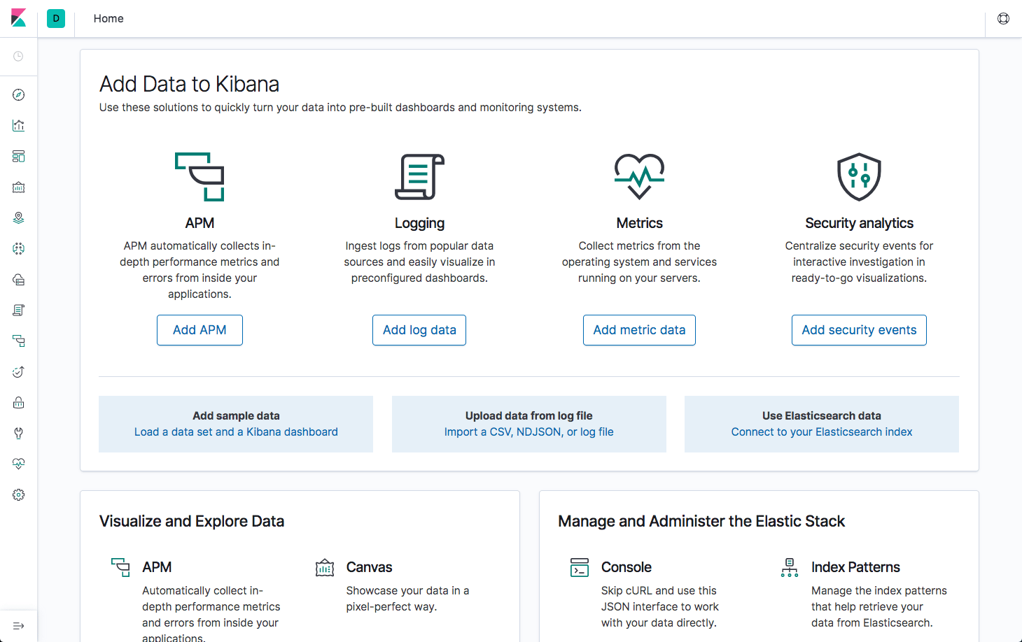
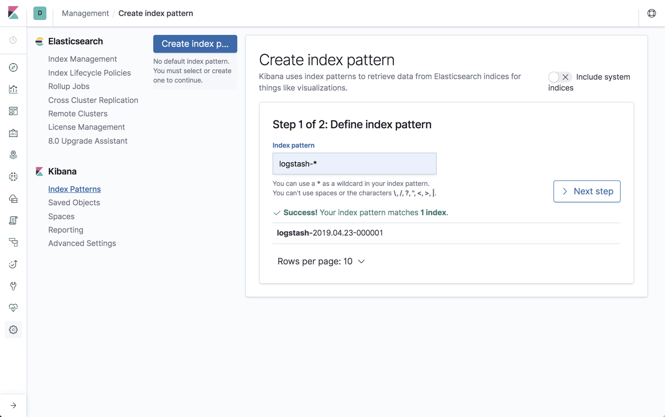
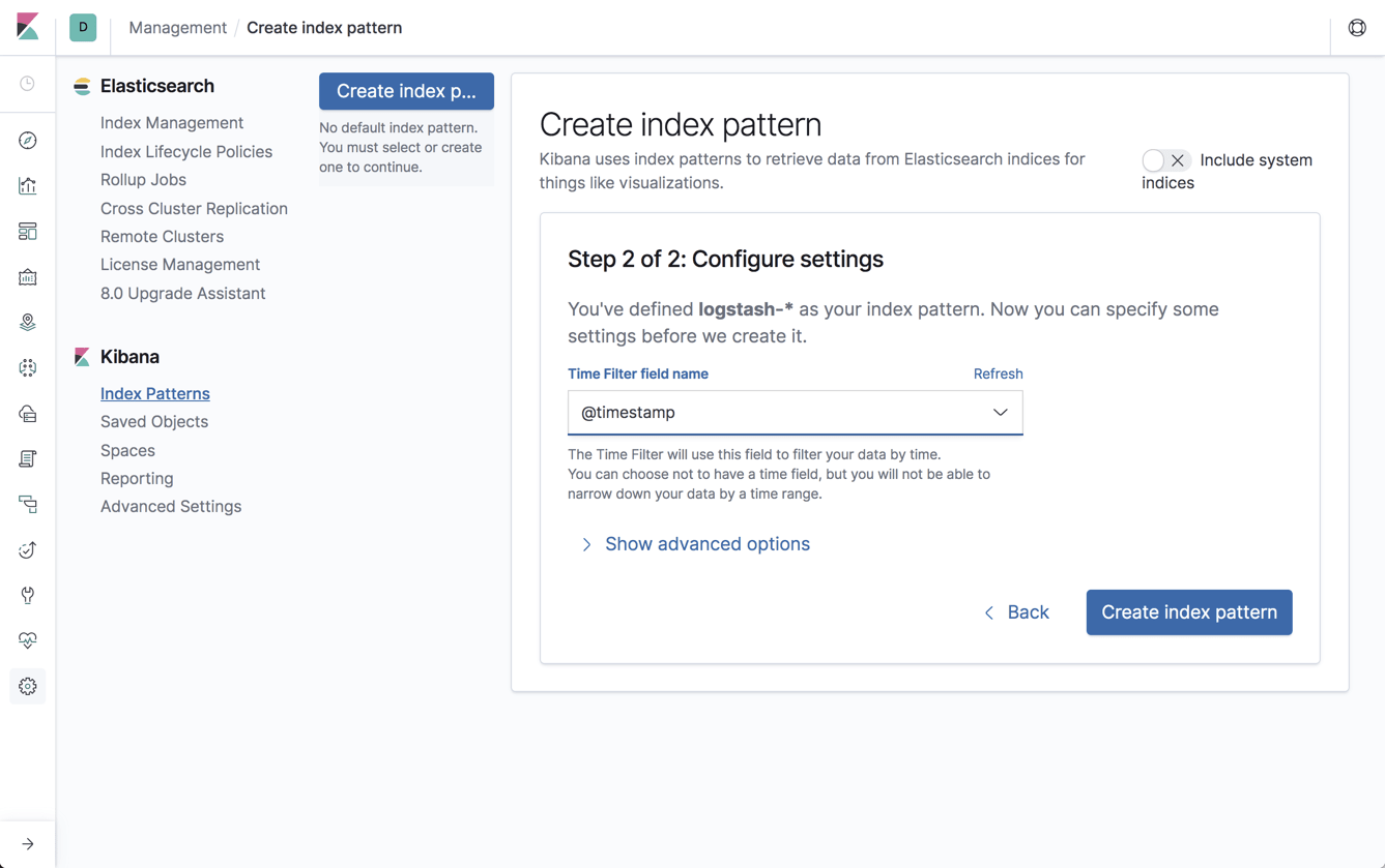
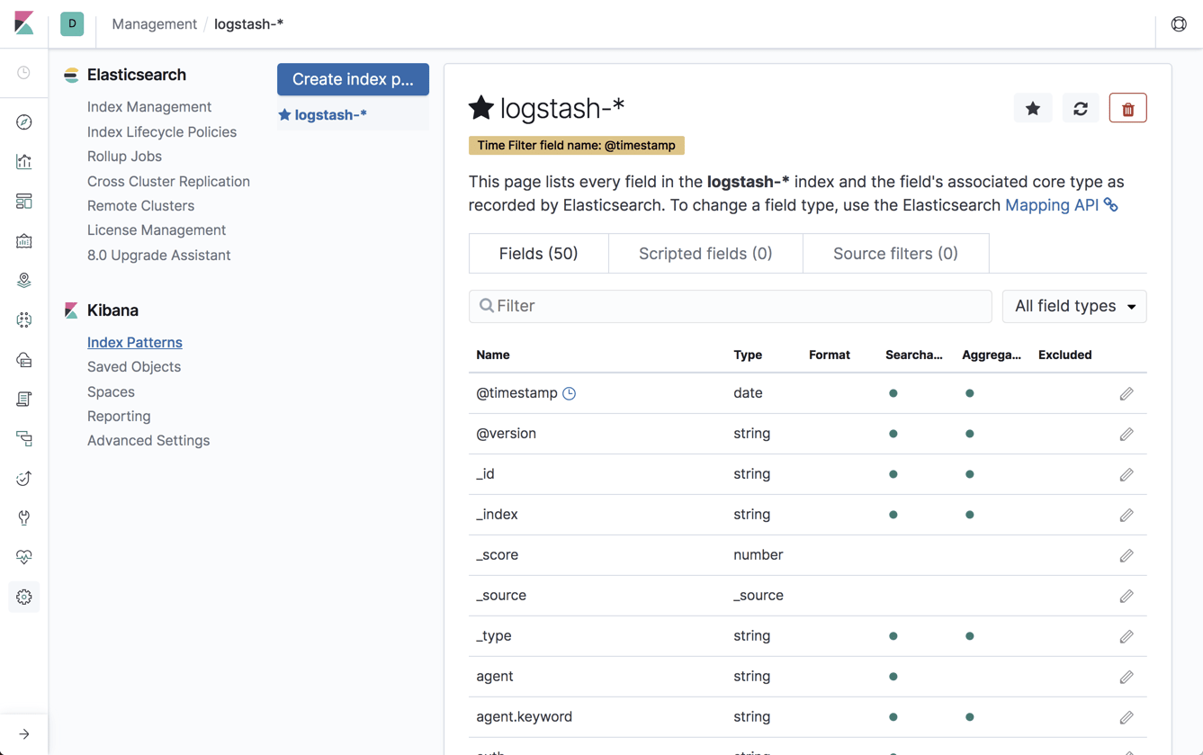
Open Kibana, define the new index patten under Management → Kibana Index Patterns, and you will begin to see the metrics collected by Metricbeat on the Discover page:

Kibana discover

Shipping to Logz.io

By making a few adjustments to the Metricbeat configuration file, you can ship the EC2 metrics to Logz.io for analysis and visualization.

First, you will need to download an SSL certificate to use encryption:

wget https://raw.githubusercontent.com/logzio/public-certificates/
master/COMODORSADomainValidationSecureServerCA.crt

sudo mkdir -p /etc/pki/tls/certs

sudo cp COMODORSADomainValidationSecureServerCA.crt 
/etc/pki/tls/certs/

Next, retrieve your Logz.io account token from the UI (under Settings → General).

Finally, tweak your Metricbeat configuration file as follows:

fields:
  logzio_codec: json
  token: <yourToken>
fields_under_root: true
ignore_older: 3hr
type: system_metrics

output.logstash:
  hosts: ["listener.logz.io:5015"]
  ssl.certificate_authorities: 
['/etc/pki/tls/certs/COMODORSADomainValidationSecureServerCA.crt']

Be sure to enter your account token in the relevant placeholder above and to comment out the Elasticsearch output.

Restart Metricbeat with:

sudo service metricbeat restart

Within a minute or two, you will see the EC2 metrics collected by Metricbeat show up in Logz.io:

33 hits

Step 4: Analyzing EC2 metrics in Kibana

Once you’ve built a pipeline of EC2 metrics streaming into your ELK Stack, it’s time to reap the benefits. Kibana offers rich visualization capabilities that allow you to slice and dice data in any way you want. Below are a few examples of how you can start monitoring your EC2 instances with visualizations.

Failed status checks

CloudWatch performs different types of status checks for your EC2 instances. Metrics for these checks can be monitored to keep tabs on the availability and status of your instances. For example, we can create a simple metric visualization to give us an indication on whether any of these checks failed:

1

CPU utilization

Kibana’s visual builder visualization is a great tool for monitoring time series data and is improving from version to version. The example below gives us an average aggregation of the ‘aws.ec2.cpu.total.pct’ field per instance.

time series

Network utilization

In the example below, we’re using the visual builder again to look at an average aggregation of the ‘aws.ec2.network.in.bytes’ field per instance to monitor incoming traffic. In the Panel Options tab, I’ve set the interval at ‘5m’ to correspond with the interval at which we’re collecting the metrics from CloudWatch.

network utilization

We can do the same of course for outgoing network traffic:

bytes out

Disk performance

In the example here, we’re monitoring disk performance of our EC2 instances. We’re showing an average of the ‘aws.ec2.diskio.read.bytes’ and the ‘aws.ec2.diskio.write.bytes’ fields, per instance:

disk performance

disk write bytes

Summing it up

The combination of CloudWatch and the ELK Stack is a great solution for monitoring your EC2 instances. Previously, Metricbeat would have been required to be installed per EC2 instance. The new AWS module negates this requirement, making the process of shipping EC2 metrics into either your own ELK or Logz.io super-simple.

Once in the ELK Stack, you can analyze these metrics to your heart’s delight, using the full power of Kibana to slice and dice the metrics and build your perfect EC2 monitoring dashboard!

ec2 monitoring dashboard

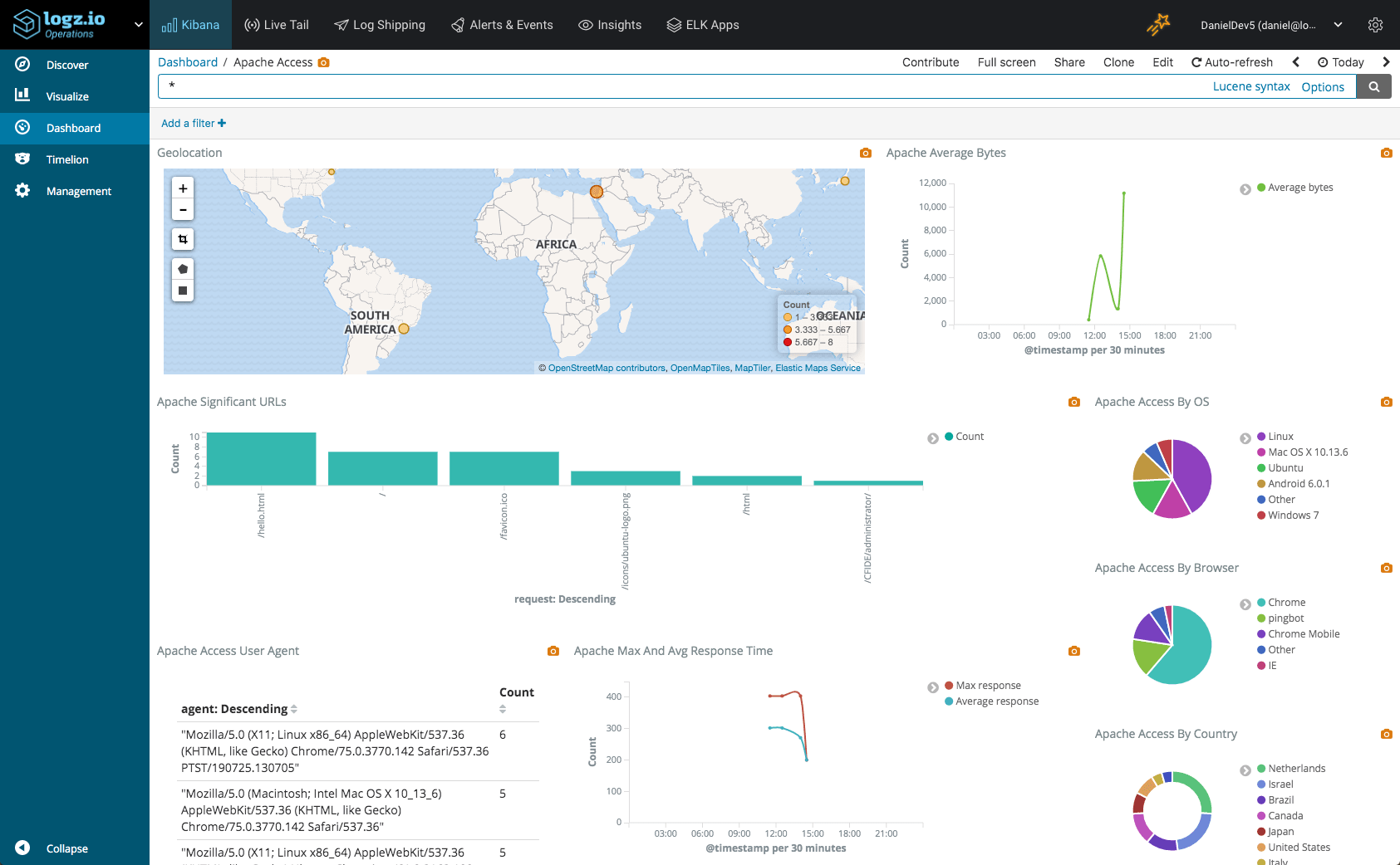
This dashboard is available in ELK Apps — Logz.io’s library of premade dashboards and visualizations for different log types. To install, simply open ELK Apps and search for ‘EC2’.

Looking forward, I expect more and more metricsets being supported by this AWS module, meaning additional AWS services will be able to be monitored with Metricbeat. Stay tuned for news on these changes in this blog!

monitoring dashboard

Easily customize your EC2 monitoring dashboard with Logz.io's ELK Apps.

Metricbeat vs. Telegraf: Side-by-Side Comparison

$
0
0

Responsible for collecting various system and service metrics and forwarding them downstream to a backend storage system, the role metric collectors play in monitoring pipelines is crucial. Despite this fact, they often get left in the shadows cast by the beautiful frontend analysis tools like Kibana or Grafana.

In the world of open source monitoring stacks, Metricbeat and Telegraf stand out as the most popular metric collectors. The truth is that they do much more than simply collect metrics. They tap into a wide variety of systems and running services, collect metrics at set intervals, execute a variety of data processing and enhancements before shipping the metrics to various different output destinations.

But which one to choose? Both were designed as part of two very different stacks, so is there even a choice to make here? This article compares the two metric collectors in an attempt to answer these questions.

Introduction

While both these collectors are native to two different monitoring stacks, ELK (Elasticsearch, Logstash and Kibana) and TICK (Telegraf, InfluxDB, Chronograf and Kapacitor), they can and should be considered separately. Both integrate with different data sources and can output to different destinations and can therefore also be used for different use cases.

Let’s start with the basics.

About Metricbeat

Metricbeat is data shipper for collecting and shipping various system and service metrics to a specified output destination. Metricbeat (previously called Topbeat) belongs to the Beats family of data shippers (Filebeat, Heartbeat, Auditbeat, etc.) and is usually used in data pipelines based on the ELK Stack. Built upon Libbeat and written in Go, Metricbeat is extremely lightweight and nimble and was designed to be easily installed and configured on edge hosts in your architecture.

About Telegraf

Telegraf is also a data shipper for collecting and shipping metrics and is most commonly used as the first component in a TICK Stack. Telegraf is also written in Go and extremely lightweight in nature. As opposed to Metricbeat, Telegraf boasts an extensive plugin ecosystem that allows users to collect metrics from a wide variety of systems, process them in a variety of ways and ship them to datastores, services,

message queues and other destinations.

Installation

Both Metricbeat and Telegraf support almost all the common installation scenarios, including all Linux-based operating systems and Windows using files or package managers. Both can also be installed with Docker using an official Docker image.

One difference is that Telegraf support for Windows is still stated as being experimental. Another difference that might matter for Kubernetes users is the availability of an official daemonset configuration which Elastic provides for Metricbeat but is not available for Telegraf. This makes it much simpler to deploy Metricbeat in a Kubernetes setup since it deploys Metricbeat per node in the cluster automatically.

Installing Metricbeat

The instructions below are for installing Metricbeat on Ubuntu with apt.

First, add the beats repository.

wget -qO - https://artifacts.elastic.co/GPG-KEY-elasticsearch | sudo 
apt-key add -

echo "deb https://artifacts.elastic.co/packages/7.x/apt stable main" | 
sudo tee -a /etc/apt/sources.list.d/elastic-7.x.list

To install an alternative package licensed under Apache 2 license, use:

echo "deb https://artifacts.elastic.co/packages/oss-7.x/apt stable main" 
| sudo tee -a /etc/apt/sources.list.d/elastic-7.x.list

Then, to install and start Metricbeat:

sudo apt-get update && sudo apt-get install metricbeat
sudo service metricbeat start

Installing Telegraf

The instructions below are for installing Telegraf on Ubuntu with apt.

First, add the InfluxData repository:

wget -qO- https://repos.influxdata.com/influxdb.key | sudo apt-key add
 -
source /etc/lsb-release
echo "deb https://repos.influxdata.com/${DISTRIB_ID,,} 
${DISTRIB_CODENAME} stable" | sudo tee 
/etc/apt/sources.list.d/influxdb.list

Then, to install and start Telegraf:

sudo apt-get update && sudo apt-get install telegraf
sudo service telegraf start

Configuration

Both Metricbeat and Telegraf are configured using a single configuration file that defines what data to collect, what to do with that data and where to ship it to. The main sections within this file follow a similar pattern, with a section for general settings and additional sections for handling inputs and outputs.

Let’s take a closer look.

Configuring Metricbeat

Metricbeat is configured using the metricbeat.yml configuration file located at:

  • Linux (DEB/RPM) – /etc/metricbeat/metricbeat.yml
  • MacOS – {extract.path}/metricbeat.yml

This file allows you to configure general Metricbeat settings as well as what modules to use. Modules define what metrics to collect and from what service. Each module specifies how to connect to the service, how often to collect the metrics, and which specific metrics to collect. Each module also has one or more metricsets which are responsible for fetching and structuring the data (see this article for a full list of these modules).

By default, Metricbeat is configured to use the system module to collect a variety of system metrics (e.g. CPU, load and memory), and ship them to a locally installed Elasticsearch instance. Additional modules can be enabled manually, using the metricbeat.yml configuration file, or using the metricbeat modules enable command. You can see a list of the modules and their default configurations under the modules.d directory (/etc/metricbeat/modules.d).

Other than defining what module to use, the metricbeat.yml configuration file can be used to tell Metricbeat how you want to handle the data. This is done using processors. For example, the drop_event processor you can drop an entire event based on an optional condition and a set of parameters.

The output section in the configuration file determines where you want to ship the metrics to. Currently, this includes Elasticsearch, Logstash, Kafka, Redis, File, Console and Elastic Cloud only.

General Metricbeat settings include a wide variety of options. You can set the name of the shipper, add tags, custom fields, and the maximum number of CPUs that can be executed simultaneously.

Metricbeat settings cannot be tested but you can use this full example of the Metricbeat configuration file can be used for reference.

Configuring Telegraf

The Telegraf configuration file is located in different locations depending on the operating system and installation type:

  • Linux (DEB/RPM) – /etc/telegraf/telegraf.conf
  • MacOS – /usr/local/etc/telegraf.conf

Telegraf also allows you to set the location of the configuration file using the –config flag and the directory of your configuration files using the –config-directory flag.

The main sections that can be configured in the Telegraf configuration file are the agent, processors, aggregators, inputs and outputs sections:

  • agent – in this section, you can configure general Telegraf settings such as the data collection interval, the batch size for metrics sent to the output plugins, the metric buffer limit, a flush interval and more.
  • processors – this section is used to define what processor plugin you want to use. Similar to Metricbeat, processor plugins in Telegraf determine how metrics are handled and processed.  
  • aggregators – this section is used to tell Telegraf what aggregator plugins you want to use. Aggregator plugins generate new aggregate metrics based on the metrics collected. For example, the ValueCounter aggregator plugin counts the occurrence of values in fields and emits the counter according to a defined schedule.
  • inputs – like the modules in Metricbeat, the inputs section in Telegraf defines which service you want to collect metrics from.
  • outputs – this is where you define what output plugin to use for shipping metrics to.

Other than the agent section, the other sections declare a specific Telegraf plugin to use, where each plugin includes specific configuration settings. Telegraf settings can be tested using the -test flag and you can use this full example of the Telegraf configuration file can be used for reference.

Pluggability

Both Metricbeat and Telegraf plug into the various systems they are monitoring and collect sets of metrics from them. Both can apply processing if required. And both then ship this data to a defined output.

The similarity ends here. The two collectors differ both in the variety of systems they can plug into and the supported output destinations with a clear advantage here for Telegraf, supporting over 200 different plugins for various systems and platforms as well as for executing processing and aggregation functions.

Inputs

Telegraf provides over 100 different input plugins whereas Metricbeat provides about 40 modules. Still, the most commonly used platforms are supported by both: containers — Kubernetes (still experimental for Telegraf) and Docker; message queues — Kafka, Redis and RabbitMQ; databases — MySQL, MongoDB, PostgreSQL and Prometheus; web servers — Apache, Nginx.

As can be expected from an ELK-native tool, Metricbeat allows users to monitor all the stack’s components — Elasticsearch, Logstash and Kibana, with dedicated modules. And vice versa, Telegraf provides an input plugin for InfluxDB.

While Metricbeat recently added support for collecting Amazon CloudWatch metrics, Telegraf has the upper hand here with support for other cloud services such as Google Pub/Sub and Amazon Kinesis.

Processors

Both collectors support multiple methods of processing, filtering and enhancing metrics before they are sent onwards to the defined output. In Metricbeat, these are called processors whereas in Telegraf they are simply processor plugins.

Both support the renaming, adding and dropping of fields. With the exception of the ability to add metadata to events using processors, it seems like Telegraf currently supports a wider variety of methods to play around with metrics.

For example, the REGEX plugin allows you to manipulate fields and change tags using REGEX expressions. The Parser plugin, in another example, allows you to parse defined fields and to create new metrics based on the contents of the field. Another interesting processor plugin is the TopK plugin, enabling users to collect the top series over a period of time.

Outputs

Here as well, Telegraf comes on top with almost 30 supported output destinations. Among these, are outputs for cloud services such as Azure Monitor, Google Stackdriver and Pub/Sub and AWS CloudWatch and Kinesis, as well as other time series databases such as Graphite, OpenTSDB and Prometheus.

As can be expected from an ELK-native tool, Metricbeat supports outputting metrics to both Elasticsearch and Logstash whereas Telegraf provides only an Elasticsearch output.

Both collectors support shipping to file and message queues — Metricbeat to both Kafka and Redis, Telegraf to Kafka only.

Performance and monitoring

Both shippers are extremely lightweight with a low resource footprint. It’s very rare, if not impossible, to encounter performance complaints.

Based on a very basic benchmark test performed on an EBS-optimized t3.2xlarge Amazon instance, with 8 vCPUs and 32 GiB memory, Metricbeat seems to have a larger footprint yet it’s still negligible in terms of overall performance. The Kibana dashboard below shows spent CPU and used memory by Metricbeat and Telegraf, both configured in this test to ship system metrics from a single host.   

performance monitoring

This is definitely not representative of how the two shippers would perform in a production environment but still might indicate a slight advantage for Telegraf.

For keeping tabs on performance, Metricbeat can be monitored using new monitoring features within Kibana (used to be an X-Pack feature). Telegraf does not provide any built-in monitoring capabilities so you are pretty much on your own here. Both shippers provide logging which can be used for troubleshooting.

Community & help

Both Metricbeat and Telegraf are pretty popular, each considered as a de-facto standard metric shipper for their respective stacks, ELK and TICK. Let’s take a look at some key indicators that can shed light as to how popular these two shippers are.   

Metricbeat

The ELK Stack is today the world’s most popular open source log analytics and log management system and this popularity has helped Metricbeat become a widely-used metric shipper. Still, Metricbeat usage remains primarily within the framework of ELK-based pipelines.

Resources: Metricbeat offers users documentation and online forums.

Stats:

  • GitHub (for all Beats): 2492 forks, 7370 stars, 9191 commits, 357 contributors.
  • Docker pulls – N/A.
  • StackOverFlow – 242 results.

metricbeat

Telegraf

Similar to Metricbeat, Telegraf’s wide usage and popularity stem from the stack it belongs to and specifically, InfluxDB. As opposed to Metricbeat though, Telegraf’s plugin ecosystem allows it to be integrated with a large number of platforms, thus extending its usage outside the TICK stack.

Resources: Telegraf offers users documentation, as well as online training, forums and a slack channel. A nice addition here is a live playground that allows users to play around with Telegraf and InfluxDB in a hosted demo environment.

Stats:

  • GitHub: 2601 forks, 6870 stars, 3947 commits, 570 contributors
  • Docker pulls: +10M pulls
  • StackOverFlow – > 500

telegraf

Summing it up

So what metric shipper to use?

From a performance perspective, both are extremely nimble with a low footprint. Both do a good job in collecting and shipping a variety of metrics, support almost the same data processing actions, and are relatively easy to configure and use.

Your decision as to which shipper to use will most likely be influenced from what monitoring stack you are using. If you’re an ELK user, Metricbeat will be the more natural choice. If you’re a TICK user, it’ll be Telegraf. However, Telegraf’s extensive plugin list makes it much more flexible, which means that you might end up using Telegraf and TICK for metrics, perhaps in combination with Grafana for analysis and visualization, and the ELK Stack for logging.

Telegraf’s Elasticsearch output plugin is limited to version 5.x so it can’t be considered for use with the ELK Stack if you’re using a current version of ELK.

Metricbeat
Telegraf
License
Apache 2.0
MIT
Size (compressed)
18.5 MB
20 MB
Modules/Plugins
40 (input only)
200+ (input, output, processor, aggregator)
Written in
Go
Go
Native stack
ELK (Elasticsearch, Logstash & Kibana)
TICK (Telegraf, InfluxDB, Chronograf and Kapacitor)
Supported OS
Linux, Windows, Mac, Docker
Build-in dashboards
Yes
No
Monitoring
Yes
No
Logging
Yes
Yes
Community & help
Docs, forums
Docs, forums, slack channel, online training, playground
Get full visibility into your system by analyzing and monitoring logs and metrics in one unified platform.

Installing the ELK Stack on Alibaba Cloud: Step by Step Guide

$
0
0

The ELK Stack is the world’s most popular open source log analytics and log management platform. Together, the four main components of the stack — Elasticsearch, Logstash, Kibana and Beats, provide users with a powerful tool for aggregating, storing and analyzing log data.

In production environments, the ELK Stack requires an infrastructure flexible and powerful enough to power it. This infrastructure needs to be scalable enough to handle data growth and bursts and preferably also be cost-efficient. Providing scalability, on-demand and high-performance resources, as well as flexible pricing models, has made the cloud a popular deployment setup for the ELK Stack.

While Amazon, and increasingly Azure, are the most common ELK deployment scenarios, other clouds are also slowly becoming popular — Google Cloud Platform, Oracle Cloud and Alibaba Cloud. In this article, we will provide instructions for setting up ELK on the latter.

Environment settings

To perform the steps below, we set up a single Alibaba Ubuntu 18.04 machine on an ecs.g5.large instance using its local storage. We set up the security group to enable access from anywhere using SSH and TCP 5601 and 9200 for accessing Kibana and Elasticsearch.

Alibaba Cloud

For more information on adding security group rules, read Alibaba’s docs here.

Accessing the Alibaba instance

Depending on your operating system and network type, there are various methods you can use to access Alibaba instances. To connect to our Ubuntu machine from my Mac, I used an SSH keypair that I created when deploying the instance. You can also use password credentials if you like.

To access the machine, first attach the required permissions to the key file:

chmod 400 <pathTofile>

And then use the following command to access:

ssh -i <pathTofile> ubuntu@<publicIP>

You should see the following output in your terminal:

Welcome to Ubuntu 18.04.2 LTS (GNU/Linux 4.15.0-48-generic x86_64)

 * Documentation:  https://help.ubuntu.com
 * Management:     https://landscape.canonical.com
 * Support:        https://ubuntu.com/advantage

Welcome to Alibaba Cloud Elastic Compute Service !

Installing Elasticsearch

The first component of the ELK Stack we will install is Elasticsearch — the heart of the stack.

First, add Elastic’s signing key so that the downloaded package can be verified (skip this step if you’ve already installed packages from Elastic):

wget -qO - https://artifacts.elastic.co/GPG-KEY-elasticsearch | sudo apt-key 
add -

Next, we need to then install the apt-transport-https package:

sudo apt-get update
sudo apt-get install apt-transport-https

We will now add the repository definition to your system:

echo "deb https://artifacts.elastic.co/packages/7.x/apt stable main" | sudo 
tee -a /etc/apt/sources.list.d/elastic-7.x.list

To install a version of Elasticsearch that contains only features license under Apache 2.0 (aka OSS Elasticsearch):

echo "deb https://artifacts.elastic.co/packages/oss-7.x/apt stable main" | 
sudo tee -a /etc/apt/sources.list.d/elastic-7.x.list

All that’s left to do is to update your repositories and install Elasticsearch:

sudo apt-get update && sudo apt-get install elasticsearch

Before we start the Elasticsearch service, we need to enter some basic Elasticsearch configurations. This is done in the Elasticsearch configuration file (On Linux: /etc/elasticsearch/elasticsearch.yml):

sudo su

vim /etc/elasticsearch/elasticsearch.yml

Since we are installing Elasticsearch on Alibaba, we will bind Elasticsearch to localhost. Also, we need to define the private IP of our instance as a master-eligible node:

network.host: "localhost"
http.port:9200
cluster.initial_master_nodes: ["<PrivateIP>"]

Save the file and run Elasticsearch with:

sudo service elasticsearch start

To confirm that everything is working as expected, point curl or your browser to http://localhost:9200, and you should see something like the following output (give Elasticsearch a minute to run):

{
  "name" : "iZt4n7jqxrkqwc2g9wqigjZ",
  "cluster_name" : "elasticsearch",
  "cluster_uuid" : "5-p-7ChvQau4TG0x9XgQzA",
  "version" : {
    "number" : "7.1.1",
    "build_flavor" : "default",
    "build_type" : "deb",
    "build_hash" : "7a013de",
    "build_date" : "2019-05-23T14:04:00.380842Z",
    "build_snapshot" : false,
    "lucene_version" : "8.0.0",
    "minimum_wire_compatibility_version" : "6.8.0",
    "minimum_index_compatibility_version" : "6.0.0-beta1"
  },
  "tagline" : "You Know, for Search"
}

Installing Logstash

Logstash requires Java 8 or Java 11 to run so we will start the process of setting up Logstash with:

sudo apt-get install default-jre

Verify java is installed:

java -version

openjdk version "11.0.3" 2019-04-16
OpenJDK Runtime Environment (build 11.0.3+7-Ubuntu-1ubuntu218.04.1)
OpenJDK 64-Bit Server VM (build 11.0.3+7-Ubuntu-1ubuntu218.04.1, mixed mode, sharing)

Since we already defined the repository in the system, all we have to do to install Logstash is run:

sudo apt-get install logstash

Before you run Logstash, you will need to configure a data pipeline. We will get back to that once we’ve installed and started Kibana.

Installing Kibana

As before, we will use a simple apt command to install Kibana:

sudo apt-get install kibana

Open up the Kibana configuration file at: /etc/kibana/kibana.yml, and make sure you have the following configurations defined:

server.port: 5601
elasticsearch.url: "http://localhost:9200"

These specific configurations tell Kibana which Elasticsearch to connect to and which port to use.

Now, start Kibana with:

sudo service kibana start

Open up Kibana in your browser with: http://localhost:5601. You will be presented with the Kibana home page (Kibana may take a minute or two to load, be patient):

Add data to Kibana


Installing Beats

The various shippers belonging to the Beats family can be installed in exactly the same way as we installed the other components.

As an example, let’s install Metricbeat:

sudo apt-get install metricbeat

To start Metricbeat, enter:

sudo service metricbeat start

Metricbeat will begin monitoring your server and create an Elasticsearch index which you can define in Kibana. In the next step, however, we will describe how to set up a data pipeline using Logstash.

More information on using the different beats is available on our blog: Filebeat, Metricbeat, Winlogbeat, Auditbeat.

Shipping some data

For the purpose of this tutorial, we’ve prepared some sample data containing Apache access logs that is refreshed daily. You can download the data here: https://logz.io/sample-data

Next, create a new Logstash configuration file at: /etc/logstash/conf.d/apache-01.conf:

sudo vim /etc/logstash/conf.d/apache-01.conf

Enter the following Logstash configuration (change the path to the file you downloaded accordingly):

input {
  file {
    path => "/home/ubuntu/apache-daily-access.log"
    start_position => "beginning"
    sincedb_path => "/dev/null"
  }
}

filter {
    grok {
      match => { "message" => "%{COMBINEDAPACHELOG}" }
    }
    date {
    match => [ "timestamp" , "dd/MMM/yyyy:HH:mm:ss Z" ]
  }
    geoip {
      source => "clientip"
    }
}

output {
  elasticsearch { 
    hosts => ["localhost:9200"] 
  }
}

Start Logstash with:

sudo service logstash start

If all goes well, a new Logstash index will be created in Elasticsearch, the pattern of which can now be defined in Kibana.

In Kibana, go to Management → Kibana Index Patterns. Kibana will automatically identify the new “logstash-*” index pattern (along with the Metricbeat index if you followed the steps for installing and running Metricbeat).

create index pattern

Enter  “logstash-*” as the index pattern, and in the next step select @timestamp as your Time Filter field.

index 2

Hit Create index pattern, and you are ready to analyze the data. Go to the Discover tab in Kibana to take a look at the data (look at today’s data instead of the default last 15 mins).

Kibana

Congratulations! You have successfully installed ELK on Alibaba and set up your first data pipeline!

What’s next?

Working with ELK involves learning the different components comprising the stack — Elasticsearch, Logstash, Kibana and Beats. The more you learn, the easier it will be to build more complex data pipelines and analyze the data itself. To help get started, I recommend reading some of the following articles on our blog:

Once your data grows, the ELK Stack can become a bit more difficult to handle. The following resources can help out with building a more resilient and scalable stack:

Enjoy!

Use the ELK you love with the cloud scalability you need.

The Definitive Guide to AWS Log Analytics Using ELK

$
0
0

Cloud is driving the way modern software is being built and deployed. At the forefront of this revolution is AWS, holding a whopping 33% of the cloud services market in Q1 2019. Considering AWS had a seven-year head start before its main competitors, Microsoft and Google, this dominance is not surprising. AWS offers, by far, the widest array of fully evolved cloud services, helping engineers to develop, deploy and run applications at cloud scale.

Applications running on AWS depend on multiple services and components, all comprising what is a highly distributed and complex IT environment. To ensure these applications are up and running at all times, performant and secure, the engineering teams responsible for monitoring these applications rely on the machine data generated by various AWS building blocks they run and depend upon. 

Needless to say, this introduces a myriad of challenges — multiple and distributed data sources, various data types and formats, large and ever-growing amounts of data — to name a few. 

Enter centralized logging 

To effectively monitor their AWS environment, users rely on a centralized logging approach. Centralized logging entails the use of a single platform for data aggregation, processing, storage, and analysis. 

  • Aggregation – the collection of data from multiple sources and outputting them to a defined endpoint for processing, storage, and analysis. 
  • Processing – the transformation or enhancement of messages into data that can be more easily used for analysis. 
  • Storage – the storage of the data in a storage backend that can scale in a cost-efficient way.
  • Analysis – the ability to monitor and troubleshoot with the help of search and visualization capabilities.

ELK to the rescue

The ELK Stack — or the Elastic Stack as it’s being called today — is the world’s most popular open source log analytics platform. An acronym for Elasticsearch, Logstash and Kibana, the different components in the stack have been downloaded over 100M times and used by companies like Netflix, LinkedIn, and Twitter.

Elasticsearch is an open source, full-text search and analysis engine, based on the Apache Lucene search engine. Logstash is a log aggregator that collects data from various input sources, executes different transformations and enhancements and then ships the data to various supported output destinations. Kibana is a visualization layer that works on top of Elasticsearch, providing users with the ability to analyze and visualize the data. And last but not least — Beats are lightweight agents that are installed on edge hosts to collect different types of data for forwarding into the stack.

Together, these different components are used by AWS users for monitoring, troubleshooting and securing their cloud applications and the infrastructure they are deployed on. Often enough, the stack itself is deployed on AWS as well. Beats and Logstash take care of data collection and processing, Elasticsearch indexes and stores the data, and Kibana provides a user interface for querying the data and visualizing it.

Using ELK for analyzing AWS environments

How ELK is used to monitor an AWS environment will vary on how the application is designed and deployed. 

For example, if your applications are running on EC2 instances, you might be using Filebeat for tracking and forwarding application logs into ELK. You might be using Mericbeat to track host metrics as well. Or, you might be deploying your applications on EKS (Elastic Kubernetes Service) and as such can use fluentd to ship Kubernetes logs into ELK. Your application might be completely serverless, meaning you might be shipping Lambda invocation data available in CloudWatch to ELK via Kinesis.

Each AWS service makes different data available via different mediums. Each of these data sources can be tapped into using various methods. Here are some of the most common methods:

  • S3 – most AWS services allow forwarding data to an S3 bucket. Logstash can then be used to pull the data from the S3 bucket in question. 
  • CloudWatch – CloudWatch is another AWS service that stores a lot of operational data. It allows sending data to S3 (see above) or streaming the data to a Lambda function or AWS Elasticsearch. 
  • Lambda – Lambda functions are being increasingly used as part of ELK pipelines. One usage example is using a Lambda to stream logs from CloudWatch into ELK via Kinesis. 
  • ELK-native shippers –  Logstash and beats can be used to ship logs from EC2 machines into Elasticsearch. Fluentd is another common log aggregator used.


Logging Pipelines

Image: Example logging pipelines for monitoring AWS with the ELK Stack.

Application logs

Application logs are fundamental to any troubleshooting process. This has always been true — even for mainframe applications and those that are not cloud-based. With the pace at which instances are spawned and decommissioned, the only way to troubleshoot an issue is to first aggregate all of the application logs from all of the layers of an application. This enables you to follow transactions across all layers within an application’s code.

There are dozens of ways to ship application logs. Again, what method you end up using greatly depends on the application itself and how it is deployed on AWS. 

For example, Java applications running on Linux-based EC2 instances can use Logstash or Filebeat or ship it directly from the application layer using a log4j appender via HTTPs/HTTP. Containerized applications will use a logging container or a logging driver to collect the stdout and stderrr output of containers and ship it to ELK. Applications orchestrated with Kubernetes will most likely use a fluentd dameonset for collecting logs from each node in the cluster.

Infrastructure logs

Everything that is not the proprietary application code itself can be considered as infrastructure logs. These include system logs, database logs, web server logs, network device logs, security device logs, and countless others. 

Infrastructure logs can shed light on problems in the code that is running or supporting your application. Performance issues can be caused by overutilized or broken databases or web servers, so it is crucial to analyze these log files especially when correlated with the application logs. 

For example, when troubleshooting performance issues ourselves, we’ve seen many cases in which the root cause was a Linux kernel issue. Overlooking such low-level logs can make forensics processes long and fruitless. 

Shipping infrastructure logs is usually done with open source agents such as rsyslog, Logstash and Filebeat that read the relevant operating system files such as access logs, kern.log, and database events. You can read here about more methods to ship logs here. The same goes for metrics, with Metricbeat being the ELK-native metric collector to use. 

infrastructure logs

AWS Service logs

As mentioned above, many AWS services generate useful data that can be used for monitoring and troubleshooting. Below are some examples, including ELB, CloudTrail, VPC, CloudFront, S3, Lambda, Route53 and GuardDuty.  

ELB Logs

Elastic Load Balancers (ELB) allows AWS users to distribute traffic across EC2 instances. ELB access logs are one of the options users have to monitor and troubleshoot this traffic.

ELB access logs are collections of information on all the traffic running through the load balancers. This data includes from where the ELB was accessed, which internal machines were accessed, the identity of the requester (such as the operating system and browser), and additional metrics such as processing time and traffic volume.

ELB logs can be used for a variety of use cases — monitoring access logs, checking the operational health of the ELBs, and measuring their efficient operation, to name a few. In the context of operational health, you might want to determine if your traffic is being equally distributed amongst all internal servers. For operational efficiency, you might want to identify the volumes of access that you are getting from different locations in the world. 

AWS allows you to ship ELB logs into an S3 bucket, and from there you can ingest them using any platform you choose. Read more about how to do this here

ELB

CloudTrail logs

CloudTrail records all the activity in your AWS environment, allowing you to monitor who is doing what, when, and where. Every API call to an AWS account is logged by CloudTrail in real time. The information recorded includes the identity of the user, the time of the call, the source, the request parameters, and the returned components. 

CloudTrail logs are very useful for a number of use cases. One of the main uses revolves around auditing and security. For example, we monitor access and receive internal alerts on suspicious activity in our environment. Two important things to remember: Keep track of any changes being done to security groups and VPC access levels, and monitor your machines and services to ensure that they are being used properly by the proper people. 

By default, CloudTrail logs are aggregated per region and then redirected to an S3 bucket (compressed JSON files). You can then use the recorded logs to analyze calls and take action accordingly. Of course, you can access these logs on S3 directly but even a small AWS environment will generate hundreds of compressed log files every day which makes analyzing this data a real challenge. 

You can read more about analyzing CloudTrail logs with the ELK Stack here.

Cloudtrail

AWS VPC Flow Logs

VPC flow logs provide the ability to log all of the traffic that happens within an AWS VPC (Virtual Private Cloud). The information captured includes information about allowed and denied traffic (based on security group and network ACL rules). It also includes source and destination IP addresses, ports, IANA protocol numbers, packet and byte counts, time intervals during which flows were observed, and actions (ACCEPT or REJECT).

VPC flow logs can be turned on for a specific VPC, VPC subnet, or an Elastic Network Interface (ENI). Most common uses are around the operability of the VPC. You can visualize rejection rates to identify configuration issues or system misuses, correlate flow increases in traffic to load in other parts of systems, and verify that only specific sets of servers are being accessed and belong to the VPC. You can also make sure the right ports are being accessed from the right servers and receive alerts whenever certain ports are being accessed. 

Once enabled, VPC flow logs are stored in CloudWatch logs, and you can extract them to a third-party log analytics service via several methods. The two most common methods are to direct them to a Kinesis stream and dump them to S3 using a Lambda function. 

You can read more about analyzing VPC flow logs with the ELK Stack here.

CloudFront Logs

CloudFront is AWS’s CDN, and CloundFront logs include information in W3C Extended Format and report all access to all objects by the CDN.

CloudFront logs are used mainly for analysis and verification of the operational efficiency of the CDN. You can see error rates through the CDN, from where is the CDN being accessed, and what percentage of traffic is being served by the CDN. These logs, though very verbose, can reveal a lot about the responsiveness of your website as customers navigate it. 

Once enabled, CloudFront will write data to your S3 bucket every hour or so. You can then pull the CloudFront logs to ELK by pointing to the relevant S3 Bucket. 

You can read more about analyzing CloudFront logs with the ELK Stack here.

cloudfront

S3 access logs

S3 access logs record events for every access of an S3 Bucket. Access data includes the identities of the entities accessing the bucket, the identities of buckets and their owners, and metrics on access time and turnaround time as well as the response codes that are returned.

Monitoring S3 access logs is a key part of securing AWS environments. You can determine from where and how buckets are being accessed and receive alerts on illegal access of your buckets. You can also leverage the information to receive performance metrics and analyses on such access to ensure that overall application response times are being properly monitored.

Once enabled, S3 access logs are written to an S3 bucket of your choice. Similar to the other AWS service logs described above, you can then pull the S3 access logs to the ELK Stack by pointing to the relevant S3 Bucket. 

S3

Lambda logs and metrics

Lambda is a serverless computing service provided by AWS that runs code in response to events and automatically manages the computing resources required by that code for the developer. 

Lambda functions automatically export a series of metrics to CloudWatch and can be configured to log as well to the same destination. Together, this data can help in gaining insight into the individual invocations of the functions. 

Shipping the data from the relevant CloudWatch log group into the ELK Stack can be done with either of the methods already explained here — either via S3 or another Lambda function. 

Route 53 logs

Route 53 is Amazon’s Domain Name System (DNS) service. Route 53 allows users to not only route traffic to application resources or AWS services, but also register domain names and perform health checks.

Route 53 allows users to log DNS queries routed by Route 53. Once enabled, this feature will forward Route 53 query logs to CloudWatch, where users can search, export or archive the data. This is useful for a number of use cases, primarily troubleshooting but also security and business intelligence.

Once in CloudWatch, Route 53 query logs can be exported to an AWS storage or streaming service such as S3 or Kinesis. Another option is to use a 3rd party platform, and this article will explore the option of exporting the logs into the ELK Stack.

You can read more about analyzing Route 53 logs with the ELK Stack here.

Route 53

GuardDuty logs

AWS GuardDuty is a security service that monitors your AWS environment and identifies malicious or unauthorized activity. It does this by analyzing the data generated by various AWS data sources, such as VPC Flow Logs or CloudTrail events, and correlating it with thread feeds. The results of this analysis are security findings such as bitcoin mining or unauthorized instance deployments.

Your AWS account is only one component you have to watch in order to secure a modern IT environment and so GuardDuty is only one part of a more complicated security puzzle that we need to decipher. That’s where security analytics solutions come into the picture, helping to connect the dots and provide a more holistic view.

GuardDuty ships data automatically into CloudWatch. To ship this data into the ELK Stack, you can use any of the same methods already outlined here — either via S3 and then Logstash, or using a Lambda function via Kinesis or directly into ELK. This article explains how to ship GuardDuty data into Logz.io’s ELK Stack using the latter.

GuardDuty

Summing it up

ELK is an extremely powerful platform and can provide tremendous value when you invest the effort to generate a holistic view of your environment. When running your applications on AWS, the majority of infrastructure and application logs can be shipped into the ELK Stack using ELK-native shippers such as Filebeat and Logstash whereas AWS service logs can be shipped into the ELK Stack using either S3 or a Lambda shipper. 

Of course, collecting the data and shipping it into the ELK Stack is only one piece of the puzzle. Some logs are JSON formatted and require little if no extra processing, but some will require extra parsing with Logstash. You can even handle processing with Lambda. Either way, parsing is a crucial element in centralized logging and one that should not be overlooked.

In addition to parsing, logging AWS with the ELK Stack involves storing a large amount of data. This introduces a whole new set of challenges — scaling Elasticsearch, ensuring pipelines are resilient, providing high availability, and so forth. To understand what it takes to run an ELK Stack at scale, I recommend you take a look at our ELK guide

Logz.io provides a fully managed ELK service, with full support for AWS monitoring, troubleshooting and security use cases. The service includes built-in integrations for AWS services, canned monitoring dashboards, alerting, and advanced analytics tools based on machine learning. 

See it for yourself--no credit card required.

Installing the ELK Stack on Mac OS X with Homebrew

$
0
0

What if I told you that it took me just under 10 minutes, 8 commands and 6 mouse clicks to create this bar chart informing me — big surprise — that I have too many open tabs in Chrome on my Mac? chart

That might sound like a lot to some readers, but if you’re not a stranger to ELK you’ll know that installing the stack, even for testing and development purposes, usually involves a whole lot more than that. 

ELK can be installed on almost any system and in any environment. Mac OS X is no exception to this rule and a new official Homebrew tap developed by Elastic makes this procedure super easy.

What is Homebrew?

Homebrew is a popular open source package manager that makes installing software on Mac OS X much simpler. Instead of downloading the bundle’s source code manually, unarchiving it, and then configuring and running it, all you have to do is enter one simple command in your CLI. 

Homebrew will download the source code, figure out if there are any dependencies, and download and compile them as well if necessary. It will then build the requested software and install it in one common location for easier access and updating. Homebrew’s inner workings and terminology are pretty straightforward but if you want to find out more, check out the docs

What makes Homebrew so popular, especially among developers, is first and foremost, its ease of use and simplicity. Coupled with extensibility, one can easily understand why it’s probably the most popular package manager for Mac.

Let’s see how the new Homebrew tap can be used to set up ELK on your Mac. 

Installing Homebrew

If you’ve already got Homebrew setup, feel free to skip to the next step. If not, here are the instructions you’ll need to install it. 

As prerequisites, you’ll need a Mac of course (preferably running Mac OS X 10.10 or later), a CLI (Terminal works just fine) and some basic command line knowledge:

cd /usr/local

/usr/bin/ruby -e "$(curl -fsSL h
ttps://raw.githubusercontent.com/Homebrew/install/master/install)"

It should take a minute or two to install, after which, run the next command to verify the installation: 

brew help

If you see some usage examples displayed, Homebrew has installed successfully. 

Installing ELK

To install the ELK Stack, we will first install the new tap containing all of the Formulae for the different components in the stack:

brew tap elastic/tap

A total of 18 formulae are “tapped” as the output message informs us:

Cloning into '/usr/local/Homebrew/Library/Taps/elastic/homebrew-tap'...
remote: Enumerating objects: 23, done.

remote: Counting objects: 100% (23/23), done.

remote: Compressing objects: 100% (23/23), done.

remote: Total 23 (delta 11), reused 10 (delta 0), pack-reused 0

Unpacking objects: 100% (23/23), done.

Checking connectivity... done.

Tapped 18 formulae (64 files, 110.0KB).

Next, we’ll install Elasticsearch, Kibana, and Metricbeat (if you want to install the open source version of these components, simply replace -full with -oss):

brew install elastic/tap/elasticsearch-full

Homebrew will download and install Elasticsearch. This might take a minute or two: 

==> Installing elasticsearch-full from elastic/tap
==> Downloading https://artifacts.elastic.co/downloads/elasticsearch/elasticsearch-7.1.1-darwin-x86_64.tar.gz?t
######################################################################## 100.0%
==> Caveats
Data:    /usr/local/var/lib/elasticsearch/elasticsearch_Daniel/
Logs:    /usr/local/var/log/elasticsearch/elasticsearch_Daniel.log
Plugins: /usr/local/var/elasticsearch/plugins/
Config:  /usr/local/etc/elasticsearch/

To have launchd start elastic/tap/elasticsearch-full now and restart at login:
  brew services start elastic/tap/elasticsearch-full
Or, if you don't want/need a background service you can just run:
  elasticsearch
==> Summary
🍺  /usr/local/Cellar/elasticsearch-full/7.1.1: 787 files, 531MB, built in 3 minutes 59 seconds

As instructed, run Elasticsearch with:

brew services start elastic/tap/elasticsearch-full

Or simply:

elasticsearch

To make sure, cURL Elasticsearch with:

curl http://localhost:9200

You should see the following output:

{
  "name" : "MacBook-Pro-4.local",
  "cluster_name" : "elasticsearch_Daniel",
  "cluster_uuid" : "x5an66f9TW6PUEqXUD9wUg",
  "version" : {
    "number" : "7.1.1",
    "build_flavor" : "default",
    "build_type" : "tar",
    "build_hash" : "7a013de",
    "build_date" : "2019-05-23T14:04:00.380842Z",
    "build_snapshot" : false,
    "lucene_version" : "8.0.0",
    "minimum_wire_compatibility_version" : "6.8.0",
    "minimum_index_compatibility_version" : "6.0.0-beta1"
  },
  "tagline" : "You Know, for Search"
}

Next, install Kibana with:

brew install elastic/tap/kibana-full

Kibana is downloaded and installed. And the output:

==> Installing kibana-full from elastic/tap
==> Downloading https://artifacts.elastic.co/downloads/kibana/kibana-7.1.1-darwin-x86_64.tar.gz?tap=elastic/homebrew-tap
######################################################################## 100.0%
==> Caveats
Config: /usr/local/etc/kibana/
If you wish to preserve your plugins upon upgrade, make a copy of
/usr/local/opt/kibana-full/plugins before upgrading, and copy it into the
new keg location after upgrading.

To have launchd start elastic/tap/kibana-full now and restart at login:
  brew services start elastic/tap/kibana-full
Or, if you don't want/need a background service you can just run:
  kibana
==> Summary
🍺  /usr/local/Cellar/kibana-full/7.1.1: 65,381 files, 407.7MB, built in 3 minutes 20 seconds

To run Kibana in the background, use: 

brew services start elastic/tap/kibana-full

Or: 

kibana

To access Kibana, open your browser at: 

http://localhost:5601

You should see Kibana’s welcome screen:

kibana

Next, let’s set up a simple data pipeline going using Metricbeat to ship some system metrics from our Mac:

brew install elastic/tap/metricbeat-full

Metricbeat is a much smaller package, so it’ll take just a few seconds to be downloaded and installed:

==> Installing metricbeat-full from elastic/tap
==> Downloading https://artifacts.elastic.co/downloads/beats/metricbeat/metricbeat-7.1.1-darwin-x86_64.tar.gz?tap=elastic/h
######################################################################## 100.0%
==> Caveats
To have launchd start elastic/tap/metricbeat-full now and restart at login:
  brew services start elastic/tap/metricbeat-full
Or, if you don't want/need a background service you can just run:
  metricbeat
==> Summary
🍺  /usr/local/Cellar/metricbeat-full/7.1.1: 38 files, 70.0MB, built in 13 seconds

Again, to start Metricbeat you can use either of the following two commands:

brew services start elastic/tap/metricbeat-full

OR

metricbeat

Within a minute or two, Metricbeat will begin shipping system metrics to Elasticsearch. You can verify by listing Elasticsearch indices:

curl -X GET "localhost:9200/_cat/indices?v"

health status index                              uuid                   pri rep docs.count docs.deleted store.size pri.store.size
yellow open   metricbeat-7.1.1-2019.06.23-000001 nfaiVJxwRCCk1z_k2nsoUA   1   1        346            0      569kb          569kb
green  open   .kibana_1                          GBiD4P-wTW-kk8zpEP5TIA   1   0          3            0     14.1kb         14.1kb
green  open   .kibana_task_manager               tnZL7bfmQ4mplwSy0YGs5g   1   0          2            0     45.5kb         45.5kb

All you need to do now to start analyzing your Mac’s performance is define the new Metricbeat index pattern in Kibana. 

Go to the management → Kibana → Index patterns page. You’ll see Kibana has automatically identified the new Elasticsearch index:

create index pattern

Define it as requested, proceed to the next step of selecting the @timestamp field, and create the new index pattern. 

You can then open the Discover page to start analyzing your data:

discover

From the list of available fields on the left, click the processname field and then the Visualize button. 

A bar chart showing the most used processes my Mac is displayed:

chart

Summing it up

I’m not great at math, but if I counted correctly, that’s eight simple commands to set up a development ELK Stack if you don’t have Homebrew installed. Two more clicks to get a useful visualization displayed! 

So, a very simple way of getting started with the ELK Stack on Mac OS X and recommended for those users playing around and just getting their feet wet. You can still install the stack using the conventional method of course, but seriously — why would you do that? 

Monitor, troubleshoot, and secure your environment with Logz.io's ELK-as-a-service.

Apache Tomcat Monitoring with ELK and Logz.io

$
0
0

Apache Tomcat is the most popular application server for serving Java applications. Widely-used, mature and well documented, Tomcat can probably be defined as the de-facto industry standard. Some sources put Tomcat’s market share at over 60%! 

Tomcat is particularly popular for serving smaller applications since it doesn’t require the full Java EE platform. It consumes a relatively small amount of resources and provides users with simpler admin features. 

Tomcat is not a web server like Apache or Nginx but is defined as a Java servlet container, or a web container that provides extended functionality for interacting with Java Servlets. But just like Apache and Nginx, Tomcat serves requests and as such provides access logs for monitoring traffic. In this article, we’ll show how to collect, process and analyze these logs using the ELK Stack and Logz.io.

To follow the steps outlined here, you’ll need your own ELK Stack or a Logz.io account. 

Tomcat logging 101

Tomcat provides a number of log types that can be used for monitoring Tomcat performance and the requests it serves:

  • Catalina log – records information about events such as the startup and shutdown of the Tomcat application server
  • Catalina.out – uncaught exceptions and thread dumps
  • Access log – records HTTP transactions between the client and the application server

As explained above, in this article we will focus on one specific type — access logs. These contain important information on the requests served by Tomcat, including the IP address of the client sending the request, the request method and URL path, the HTTP status code, the number of bytes returned to the client and more.

Step 1: Installing Tomcat

If you’ve already got Tomcat installed, great. Just skip to the next section. If you haven’t, below are instructions for installing the server on an Ubuntu 16.04 machine. Note, we’re also installing tomcat8-docs, tomcat8-examples, and tomcat8-admin which provide web apps with docs, tests, and admin features for Tomcat.  

sudo apt-get update

sudo apt-get install tomcat8
sudo apt-get install tomcat8-docs tomcat8-examples tomcat8-admin
sudo systemctl start tomcat8

As a side note, OpenJDK will be installed as a dependency when you install the tomcat8 package which will also help us when installing Logstash.

Step 2: Shipping to ELK

There are a number of ways you could ship the Tomcat access logs to the ELK Stack. You could use Logstash as the collector, processor and forwarder. If you have multiple Tomcat servers, however, a better method would be to use Filebeat as a collector on each host, and a single Logstash instance for aggregating the logs, processing them and forwarding them into Elasticsearch.

Installing and configuring Filebeat

First, and if you haven’t already, download and install the Elastic signing key: 

wget -qO - https://artifacts.elastic.co/GPG-KEY-elasticsearch | sudo 
apt-key add -

Then, save the repository definition:

echo "deb https://artifacts.elastic.co/packages/7.x/apt stable main" | sudo tee -a 
/etc/apt/sources.list.d/elastic-7.x.list

To install Filebeat, use:

sudo apt-get update 
sudo apt-get install filebeat

Next, configure Filebeat to collect the Tomcat access log file and forward it to Logstash for processing:

sudo vim /etc/filebeat/filebeat.yml
filebeat.inputs:
- type: log
  enabled: true
  paths:
    - /var/log/tomcat8/localhost_access_log.*.txt

output.logstash:
  hosts: ["localhost:5044"]

Installing and configuring Logstash

Our next part of the pipeline is Logstash. Java should already be installed if you’re running Tomcat, so simply run:

sudo apt-get install logstash

sudo apt-get install logstash:

sudo vim /etc/logstash/conf.d/tomcat8.conf

In this file, we will use the beats input plugin, a number of filter plugins to process the data including the geoip filter plugin for adding geographic data to the logs, and the Elasticsearch output plugin:

input {
  beats {
    port => 5044
    
}
 
filter {
    grok {
      match => { "message" => "%{COMBINEDAPACHELOG}" }
    
    date {
      match => [ "timestamp" , "dd/MMM/yyyy:HH:mm:ss Z" ]
    
    geoip {
      source => "clientip"
    
}
 
output {
  elasticsearch { 
    hosts => ["localhost:9200"] 
  
}

We can now start the pipeline with:

sudo service logstash start
sudo service filebeat start

Within a minute or two, you should see a new Logstash index in Elasticsearch…

curl -X GET "localhost:9200/_cat/indices?v"

health status index                      uuid                   pri rep docs.count docs.deleted store.size pri.store.size
green  open   .kibana_task_manager       8cIOckjdQr-Kz8oYoyWEZg   1   0          2            0     45.5kb         45.5kb
green  open   .kibana_1                  upsj6c9GRl6B5eU7MNvLBg   1   0          5            0     29.9kb         29.9kb
yellow open   logstash-2019.06.17-000001 hDgkiPbqRw6x5OpdZT-qtg   1   1         45            0      159kb          159kb

You can then define the “logstash-*” index pattern in Kibana under Management → Kibana → Index Patterns. Once defined, you’ll be able to start analyzing the Tomcat access logs on the Discover page:

kibana discover

Shipping to Logz.io

Since Tomcat access logs are identical to Apache access logs, shipping them into Logz.io is super simple. Logz.io provides automatic parsing, so all you need to do is install and configure Filebeat.

First, though, execute the following 3 commands to download and copy the required SSL certificate:

wget https://raw.githubusercontent.com/logzio/public-certificates/master/COMODORSADomainValidationSecureServerCA.crt
sudo mkdir -p /etc/pki/tls/certs
sudo cp COMODORSADomainValidationSecureServerCA.crt /etc/pki/tls/certs/

Next, we need to edit the Filebeat configuration file. You can configure this file manually if you like, but Logz.io provides a wizard for generating it automatically. Under Log Shipping, open the Filebeat section, and click the button to open the wizard. 

Fill in the fields as follows:

filebeat wizard

Note the type which is defined as Apache Access logs — this will ensure the Tomcat logs are processed and parsed properly.

Create the file and copy it into the /etc/filebeat folder, overriding the existing configuration file. 

Starting Filebeat, you’ll see the Tomcat logs in Logz.io appear within a minute or two:

tomcat logs

Step 3: Searching Tomcat logs

Kibana is a great tool for diving into logs and offers users a wide variety of search methods when troubleshooting. Recent improvement to the search experience in Kibana, including new filtering and auto-completion, make querying your logs an easy and intuitive experience. 

Starting with the basics, you can enter a free text search for a specific URL called by a request:

manager

manager

Or, you can use a field-level search to look for all 404 responses:

Response: 404

response 404

Using a range, you could search for all 4** responses:

response >= 400

response 400

How about all error responses originating from a specific country?

response >= 400 and geoip.country_name : "Netherlands"

1 hit

These are just some basic examples. Again, Kibana offers a wide array of querying options to choose from. Check out this article for more information on these options.

Step 4: Visualizing Tomcat logs

Of course, Kibana is renowned for its visualization capabilities and the last step in this article is to see how we can apply these capabilities to Tomcat access logs. Kibana provides almost 20 different visualization types which you can choose from. Here are some examples.

No. of requests

Use a Metric visualization, for example, for displaying single metrics. In the visualization below, we’re displaying the total no. of requests being sent. You could also breakdown this number per server in case of multiple Tomcat instances.

12,431

A line chart will help you visualize the number of requests over time:

line

Response breakdown

Another simple visualization outlines the most common response types to requests. We could use various visualization types for this, but here we’re using a pie chart:

cirlce

Top requests

It’s always interesting to monitor what URLs are being called the most. To visualize this, we can use a Data Table visualization:

status

Requests map

Where are request coming from? This is especially important for security reasons but also for infrastructure optimization. We’re using a Coordinate Map visualization that uses the geo-enhanced fields in the Tomcat access logs:

map

Once you have your visualizations lined up, you can add them all up into one beautiful Kibana dashboard:

dashboard

This dashboard is available for use in ELK Apps — our free library of premade dashboards, visualizations and alerts for different log types. If you’re a Logz.io user, simply open the ELK Apps page and search for ‘Tomcat’ for an easy 1-click install.

Endnotes

Tomcat access logs provide valuable information on the traffic being served. The ELK Stack allows you to aggregate the logs, process them, and of course, analyze them using queries and visualizations. 

Of course, access logs are just one part of the puzzle. For accurately gauging Tomcat performance, these logs should be combined together with Tomcat’s Catalina logs and JMX metrics. Together, these data sources will provide you with a more complete picture on how Tomcat is performing and we will look into using these additional data sources in the articles in this series. 

Easily monitor Tomcat performance with Logz.io.


Distributed Tracing with Jaeger and the ELK Stack

$
0
0

Over the past few years, and coupled with the growing adoption of microservices, distributed tracing has emerged as one of the most commonly used monitoring and troubleshooting methodologies. 

New tracing tools and frameworks are increasingly being introduced, driving adoption even further. One of these tools is Jaeger, a popular open source tracing tool. This article explores the integration of Jaeger with the ELK Stack for analysis and visualization of traces.

What is Jaeger?

Jaeger was developed by Uber and open sourced in 2016. Inspired by other existing tracing tools, Zipkin and Dapper, Jaeger is quickly becoming one of the most popular open source distributed tracing tools, enabling users to perform root cause analysis, performance optimization and distributed transaction monitoring.  

Jaeger features OpenTracing-based instrumentation for Go, Java, Node, Python and C++ apps, uses consistent upfront sampling with individual per service/endpoint probabilities, and supports multiple storage backends — Cassandra, Elasticsearch, Kafka and memory.

From an architectural perspective, Jaeger is comprised of multiple components, three of which provide the core backend functionality: Jaeger Clients implement OpenTracing API in applications, creating spans when receiving new requests. Jaeger Agents are responsible for listening for spans and sending them to the Collector.  The collector, in turn, receives the traces from the agents and runs them through a processing pipeline which ends with storing them in backend storage. 

Jaeger and ELK

The default storage is Cassandra but Jaeger can also store traces in Elasticsearch. This capability means users can analyze traces using the full power of the ELK Stack (Elasticsearch, Logstash and Kibana). Why does this matter?

Sure, Jaeger ships with a nifty GUI that allows users to dive into the traces and spans. Using the ELK Stack, though, offers users additional querying and visualization capabilities. Depending on your ELK architecture, you will also be able to store trace data for extended retention periods. If you’re already using the ELK Stack for centralized logging and monitoring, why not add traces into the mix?

Let’s take a closer look at how to set up the integration between Jaeger and the ELK Stack and some examples of what can be done with it. 

Step 1: Setting Up Elasticsearch and Kibana

Our first step is to set up a local ELK (without Logstash) with Docker. Jaeger currently only supports versions 5.x and 6.x, so I will use the following commands to run Elasticsearch and Kibana.

Elasticsearch 6.8.0:

docker run --rm -it --name=elasticsearch -e "ES_JAVA_OPTS=-Xms2g -Xmx2g" 
-p 9200:9200 -p 9300:9300 -e "discovery.type=single-node" -e 
"xpack.security.enabled=false" 
docker.elastic.co/elasticsearch/elasticsearch:6.8.0

Kibana 6.8.0:

docker run --rm -it --link=elasticsearch --name=kibana -p 5601:5601 
docker.elastic.co/kibana/kibana:6.8.0

Step 2: Setting Up Jaeger

Next, we will deploy Jaeger.

Designed for tracing distributed architectures, Jaeger itself can be deployed as a distributed system. However, the easiest way to get started is to deploy Jaeger as an all-in-one binary that runs all the backend components in one single process.

To do this, you can either run the jaeger all-in-one binary, available for download here, or use Docker. We will opt for the latter option.

Before you copy the command below, a few words explaining some of the flags I’m using:

  • –link=elasticsearch – link to the Elasticsearch container.
  • SPAN_STORAGE_TYPE=elasticsearch – defining the Elasticsearch storage type for storing the Jaeger traces.
  • -e ES_TAGS_AS_FIELDS_ALL=true – enables correct mapping in Elasticsearch of tags in the Jaeger traces.

docker run --rm -it --link=elasticsearch --name=jaeger -e 
SPAN_STORAGE_TYPE=elasticsearch -e 
ES_SERVER_URLS=http://elasticsearch:9200 -e ES_TAGS_AS_FIELDS_ALL=true 
-p 16686:16686 jaegertracing/all-in-one:1.12

You can now browse to the Jager UI with: http://localhost:16686

beaver

Step 3: Simulating trace data

Great, we’ve got Jaeger running. It’s now time to create some traces to verify they are being stored on our Elasticsearch instance. 

To do this, I’m going to deploy HOT R.O.D  – an example application provided as part of the project that consists of a few microservices and is perfect for easily demonstrating Jaeger’s capabilities.

Again, using Docker:

docker run --rm --link jaeger --env 
JAEGER_AGENT_HOST=jaeger --env JAEGER_AGENT_PORT=6831 -p8080-8083:8080-8083 
jaegertracing/example-hotrod:latest all

Open your browser at: http://localhost:8080:

hot rod

Start calling the different services by playing around with the buttons in the app. Each button represents a customer and by clicking the buttons, we’re ordering a car to the customer’s location. Once a request for a car is sent to the backend, it responds with details on the car’s license plate and the car’s ETA:

rod data

Within seconds, traces will be created and indexed in Elasticsearch. 

To verify, cURL Elasticsearch:

curl -X GET "localhost:9200/_cat/indices?v"

health status index                     uuid                   pri rep docs.count docs.deleted store.size pri.store.size
green  open   .kibana_1                 LffR3embTkyjs-TdCMQYYQ   1   0          4            0     14.4kb         14.4kb
yellow open   jaeger-span-2019-06-18    Vuujr66CTg6AdPgPkX7xUw   5   1          1            0     11.4kb         11.4kb
green  open   .kibana_task_manager      btmJCT9MQ9ydviiMWgDxCQ   1   0          2            0     12.5kb         12.5kb
yellow open   jaeger-service-2019-06-18 T_lS1JQWT4aozUHxVmY9Tw   5   1          1            0      4.5kb          4.5kb

Step 4: Hooking up Jaeger with ELK

The final step we need to take before we can start analyzing the traces is define the new index pattern in Kibana.

To do this, open the Management → Kibana → Index Patterns page. Kibana will display any Elasticsearch index it identifies, including the new Jaeger index.  

Kibana index pattern

Enter ‘jaeger-span-*’ as your index pattern, and in the next step select the ‘statTimeMillis’ field as the time field.

step 2

Hit the Create index pattern button and then open the Discover page — you’ll see all your Jaeger trace data as indexed and mapped in Elasticsearch:

discover

Step 5: Analyzing traces in Kibana

You can now start to use Kibana queries and visualizations to analyze the trace data. Kibana supports a wide variety of search options and an even bigger amount of visualization types to select from. Let’s take a look at some examples.

No. of traces

Let’s start with the basics. Metric visualizations are great for displaying a single metric. In the examples below we’re showing the overall number of traces being sampled:

traces

Traces per service

Using a bar chart visualization, we can view a breakdown of the traces per microservice. To build this visualization, use a count aggregation as the Y axis, and a terms aggregation of the process.serviceName field as the X axis.

graph

Avg. transaction duration

Line charts are useful for identifying trends over time. In the example below, we’re using a line chart to monitor the average duration of requests per service. To build this visualization, use an average aggregation of the duration field as the Y axis, together with a time histogram and a split series of the process.serviceName field as the Y axis:

span types

Span types

Pie charts are super simple visualizations that can help view a breakdown of a specific field. In the example below, we’re using a pie chart to visualize the breakdown between client and server requests using a terms aggregation of the tag.span@kind field:

pie

Trace list

Using a saved search visualization, you can insert a list of the actual traces as a visualization in a dashboard. To do this, first save the search in the Discover page. In the example below, I’ve added the duration, process.serviceName, spanID and operationName fields to the main view but you can, of course, add the fields you want to be displayed:

list

Then, when adding visualizations to your dashboard simply select to add a visualization from a saved search and select the search you saved above.

Adding this visualization, together with all the other visualizations, in one dashboard gives you a nice overview of all the tracing activity Jaeger has recorded and stored in Elasticsearch:

dashboard

Endnotes

The Jaeger UI does a great job at mapping the request flow, displaying the different spans comprising traces and allowing you to drill down into them. You can even compare different traces to one another. 

Kibana provides users with additional querying and visualization capabilities which give you with a more comprehensive view. Again, when combined with logs and metrics — using the ELK Stack with Jaeger is a powerful combination. 

We recently introduced an integration for Zipkin, allowing Logz.io users to analyze their traces together with their logs and metrics in one platform. Jaeger is next on our list so stay tuned! 

Get complete visibility into your systems by analyzing logs, metrics, and traces in one unified platform.

Using the Mutate Filter in Logstash

$
0
0

One of the benefits of using Logstash in your data pipelines is the ability to transform the data into the desired format according to the needs of your system and organization. There are many ways of transforming data in Logstash, one of them is using the mutate filter plugin.

This Logstash filter plugin allows you to force fields into specific data types and add, copy, and update specific fields to make them compatible across the environment. Here’s a simple example of using the filter to rename an IP field HOST_IP.

...
mutate { 
  rename => { “IP” => “HOST_IP” } 
}
...

In this article, I’m going to explain how to set up and use the mutate filter using three examples that illustrate the types of field changes that can be executed with it.

The basics

The mutate filter plugin (a binary file) is built into Logstash. You can verify that with the following commands:

cd /usr/share/logstash/bin
./logstash-plugin list | grep -i mutate

The output will be:  

logstash-filter-mutate

The mutate filter and its different configuration options are defined in the filter section of the Logstash configuration file. The available configuration options are described later in this article. Before diving into those, however, let’s take a brief look at the layout of the Logstash configuration file.

Generally, there are three main sections of a Logstash configuration file: 

  • Input – this is where the source of data to be processed is identified. 
  • Filter – this is where the fields of the incoming event logs can be transformed and processed. 
  • Output – this is where parsed data will be forwarded to.

More information about formatting the Logstash configuration file can be found here.

In the example below, we’re adding a tag (Apache Web Server) to incoming apache access logs with a condition that the source path contained the term “apache”. Note the mutate filter added in the filter section of the Logstash configuration file:

input {
  file {
    path => "/var/log/apache/apache_access.log"
    start_position => "beginning"
    sincedb_path => "NULL" }
}
filter {	
	if [ source ] =~ /apache/ {
   mutate {
                add_tag => [ "Apache Web Server" ] }
}}

output {
  elasticsearch { hosts => ["localhost:9200"] }
}

Mutate Filter Configuration Options 

There are a number of configuration options which can be used with the mutate filter, such as copy, rename, replace, join, uppercase, and lowercase. 

They are outlined in the table below: 

Configuration Options
Usage
add_field
add a new field to the event
remove_field
remove an arbitrary field from the event
add_tag
add an arbitrary tag to the event
remove_tag
remove the tag from the event if present
convert
convert the field value to another data type
id
add a unique id to the field event
lowercase
convert a string field to its lowercase equivalent
replace
replace the field with the new value
strip
remove the leading and trailing white spaces
uppercase
convert a string field to its uppercase equivalent
update
update an existing field with new value
rename
rename a field in the event
gsub
for find and replace substitution in strings
merge
to merge the array or hash events

Simple and Conditional Removals

Performing a Simple Removal

In this example, we want to remove the “Password” field from a small CSV file with 10-15 records. This type of removal can be very helpful when shipping log event data that includes sensitive information. Payroll management systems, online shopping systems, and mobile apps handling transactions are just a few of the applications for which this action is necessary.

password 1

The configuration below will remove the field “Password”:

input {
  file {
    path => "/Users/put/Downloads/Mutate_plugin.CSV"
    start_position => "beginning"
    sincedb_path => "NULL"
  }
}

filter {
  csv { autodetect_column_names => true }
  mutate { 
	remove_field => [ "Password" ] }
}

output {
  stdout { codec => rubydebug }
}

After the code has been added, run the Logstash config file. In this case, the final outcome will be shown in the terminal since we are printing the output on stdout. 

As seen below, the “Password” field has been removed from the events:

Christi

Performing a Conditional Removal

In this example, the field “Password” is again being removed from the events. This time, however, the removal is conditioned by the salary, if [Salary] == “154216.”

password2


The code below will remove the field “Password” using the condition specified earlier:

input {
  file {
    path => "/Users/put/Downloads/Mutate_plugin.CSV"
   start_position => "beginning"
   sincedb_path => "NULL"
  } }

filter {
  csv { autodetect_column_names => true }
  if [Salary] == "154216" {
	mutate { 
	  remove_field => [ "City" ] } }	
}

output {
  stdout { codec => rubydebug }
}

Now, run Logstash with this configuration code. The result of this conditional removal is shown below:

users

Merging Fields

In this example, we’re going to use the mutate filter to merge two fields, “State” and “City” using the MERGE option. 

After merging the two, the “State” field will have the merged data in an array format. In addition, in order to make things clear, we will also RENAME the field as shown in the code below:

input {
  file {
    path => "/Users/put/Downloads/Mutate_plugin.CSV"
    start_position => "beginning"
   sincedb_path => "NULL"  }}

filter {
  csv { autodetect_column_names => true }

  mutate {
                merge => { "State" => "City" } }

  mutate {
                rename => [ "State" , "State-City" ]  } }

output {
  stdout { codec => rubydebug }
}

Run the Logstash config file shown below to yield the merged data as shown below:

state city

Adding White Spaces

Next, we’re going to use the mutate filter to add white spaces to the “message” field of incoming events. Currently, there is no space in the values of the “message” field. We will use mutate filter’s “GSUB” option as shown in the code below:

input {
  file {
    path => "/Users/put/Downloads/Mutate_plugin.CSV"
    start_position => "beginning"
   sincedb_path => "NULL"
  }
}

filter {
  csv { autodetect_column_names => true }
  
  mutate {
	 gsub => [ "message", "," , ", " ] 
	 }
 }

output {
  stdout { codec => rubydebug }
}

Run the Logstash configuration to see the added white spaces in the message field, as shown below:

message

Endnotes

This article has demonstrated how a mutate filter can create new fields in a data set as well as replace and rename existing fields. There are many other important filter plugins in Logstash which can also be useful while parsing or creating visualizations. 

Some of these include:

  • JSON—used to parse the JSON events.
  • KV—used to parse the key-value pairs.
  • HTTP—used to integrate external APIs.
  • ALTER—used to alter fields which are not handled by a mutate filter.

You can learn more about these plugins in this article.

Get all the benefits of ELK without the burden of maintaining it.

A Guide to Open Source Monitoring Tools

$
0
0

Open source is one of the key drivers of DevOps. The need for flexibility, speed, and cost-efficiency, is pushing organizations to embrace an open source-first approach when designing and implementing the DevOps lifecycle. 

Monitoring — the process of gathering telemetry data on the operation of an IT environment to gauge performance and troubleshoot issues — is a perfect example of how open source acts as both a driver and enabler of DevOps methodologies. Today, engineers can select from a huge and ever-growing number of open source tools to help them with various elements involved in monitoring–from databases, to user interfaces, to instrumentation frameworks, to data collectors and monitoring agents — you name it.

This poses somewhat of a challenge. Is there a difference between systems for logs and metrics? What’s a time-series database? Can log management also be considered part of monitoring? These are just some questions engineers face when trying to build a telemetry system for monitoring their environment. 

There are a lot of buzzwords being thrown about (did anyone say observability?) and it’s easy to get confused. The goal of the list below is to try and help those getting started with monitoring understand the different options available in the market.

Some disclaimers

Before we get started, I wanted to clarify the scope of the list to set some expectations:

  • Yes, there are other tools: This is by no means an exhaustive list of all the open source monitoring tools in the market. The tools listed here are some of the most popular ones used for monitoring cloud-native applications and as such, are most likely already being used by a large number of our readers. Still, I’ve probably omitted some popular tools so please feel free to mention these in the comments below and I’ll do my best to add them to the list.
  • Define monitoring please!  You’ll notice the list includes tools used for more than just metric collection and analysis. There are plenty of definitions of the term “monitoring” but I’m purposely using a more inclusive interpretation to include logging, alerting and tracing tools. Monitoring involves many different steps — data collection, data processing, data analysis — to name just a few. The tools listed here take care of one or more of these steps.  

Let’s get started.

Grafana

Grafana is an extremely popular (almost 30,000 stars on GitHub!) open source data analysis and visualization tool, notorious for the beautiful sleek monitoring dashboards that can be built with it. Here’s a taste:

Grafana

 This is only one reason why Grafana is so popular. Another major reason is its ability to work together with a very large number of data sources. The list of supported data sources includes Graphite, Prometheus, InfluxDB, Elasticsearch, PostgreSQL, MySQL, Google Stackdriver, Azure Monitor, and more.  Plugins make Grafana more extendable, enabling users of a long list of other systems to integrate with Grafana (yes, there is also a Logz.io plugin).

Grafana is extremely robust, featuring a long list of capabilities such as alerts, annotations, filtering, data source-specific querying, visualization and dashboarding, authentication/authorization, cross-organizational collaboration, and plenty more. 

Grafana is pretty easy to install and use, and most deployments are performed by users whether on-prem or on the cloud. There are, however, some hosted Grafana solutions, designed to take away some of the management headache involved in running Grafana. It’s also worth pointing out that while Grafana was designed for metrics analysis, recent developments (namely, Loki) seem to be leading Grafana into the direction of log analysis as well.

Pros: Large ecosystem, rich visualization capabilities

Cons: Cannot (currently) be used to analyze logs

Prometheus

Up until about 7 years ago, Prometheus was the name of a Titan in Greek mythology. SoundCloud changed that with the development, and open sourcing, of what has now become one of the most popular systems and service monitoring tools today. 

Prometheus is comprised of multiple components, the core of the system being the Prometheus server that scrapes and stores metrics. A variety of client libraries are available for all the popular languages and runtimes, including Go, Java/JVM, C#/.Net, Python, Ruby, Node.js, Haskell, Erlang, and Rust. Also worth mentioning are the push gateway for supporting short-lived jobs, the alert manager for handling alerts and exporters for exposing metrics from 3rd party systems in a non-Prometheus format (e,g, MongoDB, Elasticsearch, CouchDB, and more).  

prometheus

Source: Prometheus

What makes Prometheus unique among other monitoring tools is a multi-dimensional data model in which metrics are identified with a name and an unordered set of key-value pairs called labels. The native querying language, PromQL, can be used to not only aggregate across these labels and then later visualize the data but also to define alerts.

Another unique and important feature of Prometheus is the pull model in which metrics are pulled over HTTP as opposed to being pushed into the system as in most monitoring systems. Meaning, to ship metrics into Prometheus, your services need to expose an endpoint. Service discovery options will help find services and start retrieving metrics from them. 

Prometheus was designed for high performance, is relatively easy to install and operate, and can be integrated into existing infrastructure components such as Kubernetes. Of course, Prometheus becomes more challenging to handle at scale and in large deployments. As stated in the docs, Prometheus’s local storage is limited by single nodes in its scalability and durability and that’s why integrating with remote storage systems is supported. Adding high availability into the mix adds another level of complexity. 

Pros: Kubernetes-native, simple to use, huge community

Cons: Challenges at scale, long-term storage

Graphite 

Graphite is another open source monitoring system designed and used for storing metrics and visualizing them. Much older than Prometheus, Graphite was originally designed by Chris Davis at Orbitz in 2006 as a side project and was subsequently open sourced in 2008. After that, it became quite popular and is still used by a large number of organizations, including Etsy, Lyft and yes — us here at Logz.io. 

Graphite is written in Python and comprised of three main components: a service called Carbon that listens for metrics being collected, a simple database library called Whisper for storing the metrics, and a Graphite web app for visualizing them. 

Graphite first set out to be scalable and highly performant to support real-time analysis — it scales horizontally and provides built-in caching — but like many open source monitoring backends starts to feel pressure under large workloads and requires careful planning around I/O, CPU and of course disk capacity.  

As a mature solution, and also probably as a result of its limited mission statement, there are a lot of tools that integrate with Graphite — from metric collectors and forwarders to alerting tools, and of course user interfaces for querying and visualizing metrics. For the latter, Grafana is by far the most popular interface for analyzing metrics stored on Graphite. 

Pros: Only handles metrics storage and rendering

Cons: Challenges at scale, only handles merics storage and rendering 

InfluxDB

InfluxDB is another open source database designed for storing metrics. Developed and maintained by InfluxData, InfluxDB is the core component of a larger stack called TICK (Telegraf, InfluxDB, Chronograf and Kapacitor) but is used extensively on its own, often together with other open source tools listed here such as Grafana.  

InfluxDB

Source: InfluxData

Two characteristics make InfluxDB one of the most popular time-series databases used today — high performance and an SQL-like querying language. Downsampling and data compression enables the handling of a large number of data points at a high rate. InfluxDB has published benchmarks proving its superior performance compared to other databases in the market and there are plenty of testimonials on the web attesting to this characteristic as well. 

Similar to Prometheus, the InfluxDB data model is also multi-dimensional, with key-value pairs called tags and a second level of labels called fields. 

Written in Go and compiled into a single binary with no external dependencies, InfluxDB is extremely easy to install. Depending on the operating system, you can either use a package manager or download the binaries and install it manually. For high availability in large production environments, InfluxDB has one big downside — clustering is only available in the commercial version.

Pros: Performance, easy-to-use API and querying

Cons: Clustering not open source

Fluentd

We all love dashboards. But while analysis and visualization tools such as Grafana and Kibana bask in glory, there is a lot of heavy lifting being done behind the scenes to actually collect the data. For logs, this heavy lifting is performed by log forwarders, aggregators and shippers. 

These tools handle the tasks of pulling and receiving the data from multiple systems, transforming it into a meaningful set of fields, and eventually streaming the output to a defined destination for storage.

Fluentd is an open source log collector, processor and aggregator that was created back in 2011 by the folks at Treasure Data. Written in Ruby, Fluentd was created to act as a unified logging layer — a one stop component that can aggregate data from multiple sources, unify the differently formatted data into JSON objects, and route it to different output destinations. 

Design wise — performance, scalability and reliability are some of Fluentd’s outstanding features. A vanilla Fluentd deployment will run on ~40MB of memory and is capable of processing above 10,000 events per second. Adding new inputs or outputs is relatively simple and has little effect on performance. Fluentd uses disk or memory for buffering and queuing to handle transmission failures or data overload and supports multiple configuration options to ensure a more resilient data pipeline. 

Fluentd has been around for some time now and has developed a rich ecosystem consisting of more than 700 different plugins that extend its functionality. Fluentd is the de-facto standard log aggregator used for logging in Kubernetes and is one of the widely used Docker images. 

We’ll be mentioning Logstash later on in this list but if all this sounds somewhat similar to what Logstash has to offer, you’re not wrong. Flunend can be considered in many ways a sequel of Logstash. There are of course some differences, and I cover some of these in this article

Pros: Huge plugin ecosystem, performance, reliability

Cons: Difficult to configure

Jaeger

Over the past few years, and coupled with the growing adoption of microservices, distributed tracing has emerged as a monitoring and troubleshooting best practice. As part of this trend and reinforcing it perhaps, are new tracing tools such as Jaeger.

Jaeger was developed by Uber and open sourced in 2016. Inspired by other existing tracing tools, Zipkin and Dapper, Jaeger is quickly becoming one of the most popular open source distributed tracing tools, enabling users to perform root cause analysis, performance optimization and distributed transaction monitoring.  

Jaeger features OpenTracing-based instrumentation for Go, Java, Node, Python and C++ apps, uses consistent upfront sampling with individual per service/endpoint probabilities, and supports multiple storage backends — Cassandra, Elasticsearch, Kafka and memory.

Jaeger

Illustration of a Jaeger architecture with Kafka acting as an intermediate buffer. Source: Jaeger docs.

From an architectural perspective, Jaeger is comprised of multiple components, three of which provide the core backend functionality: Jaeger Clients implement OpenTracing API in applications, creating spans when receiving new requests. Jaeger Agents are responsible for listening for spans and sending them to the Collector.  The collector, in turn, receives the traces from the agents and runs them through a processing pipeline which ends with storing them in backend storage. 

Pros: User interface, various instrumentation options

Cons: Limited backend integration

ELK 

You didn’t think I’d end this article without mentioning ELK, right?

The ELK Stack (also known as the Elastic Stack) is today the world’s most popular log management and log analysis platform in the market used for monitoring, troubleshooting and security use cases. While the stack is primarily used for logs, recent changes in Elasticsearch and new analysis capabilities in Kibana are making it more and more popular for metrics as well.

The stack is comprised of 3 main components: Elasticsearch, Logstash, and Kibana. Elasticsearch is the stack’s data store, Logstash is a log aggregator and processor and Kibana is a user interface used for analysis.  A 4th component is Beats — a family of lightweight data shippers used for shipping different data types into the stack.   

There are a number of reasons ELK is so popular, the fact that the stack is open source being only one. Elasticsearch was designed for scalability and can perform extremely well even when storing, and searching across, a very large amount of documents. A rich RESTful API makes it extremely easy to work with. Kibana is an extremely versatile analysis tool supporting various different ways of slicing and dicing data. 

ELK comes with its own set of challenges, of course, especially at scale.  This is why there are hosted solutions such as AWS Elasticsearch and Elastic’s Elasticsearch service and a fully managed service such as Logz.io. You can understand the key differences between these options here. 

Pros: Huge community, easy to deploy and use, rich analysis capabilities

Cons: Challenges at scale

Endnotes

It’s hard to overestimate the contribution of open source monitoring tools to software development. As articulated in the intro to this list, open source is both a key driver and an enabler of modern development methodologies and DevOps specifically that require speed, flexibility and extensibility. 

As great as open source tools are, they are not without challenges. To paraphrase Tolkien, not all that is open source is actually free. Yes, the monitoring tools listed above will not require a credit card or a purchase order. But at scale, and when deployed in production, they will most likely cost your organization in terms of the time and resources required to deploy and maintain over time. 

This is something to consider when planning your telemetry system. IT environments are only getting more complex and you need to think carefully before adding another layer of complexity to your day-to-day work.  

I hope to be slowly adding more and more open source monitoring tools to this list, and like I said — feel free to comment below to suggest which tools these should be.

Happy monitoring!

Logz.io offers ELK and Grafana in one unified platform for monitoring, troubleshooting, and security.

Deploying Redis with the ELK Stack

$
0
0

In a previous post, I explained the role Apache Kafka plays in production-grade ELK deployments, as a message broker and a transport layer deployed in front of Logstash. As I mentioned in that piece, Redis is another common option. I recently found out that it is even more popular than Kafka!  

Known for its flexibility, performance and wide language support, Redis is used both as a database and cache but also as a message broker. For ELK-based data pipelines, Redis can be placed between Beats and Logstash, as a buffering layer, giving downstream components better chances of processing and indexing the data successfully.

In this article, I’ll show how to deploy all the components required to set up a data pipeline using the ELK Stack and Redis: 

  • Filebeat – to collect logs and forward them to Redis 
  • Redis – to brokers the data flow and queue it
  • Logstash – to subscribe to Redis, process the data and ship it to Elasticsearch
  • Elasticsearch – to index and store the data
  • Kibana – to analyze the data.

beats to redis

My setup 

I installed all the pipeline components on a single Ubuntu 18.04 machine on Amazon EC2 using local storage. Of course, in real-life scenarios you will probably have some or all of these components installed on separate machines. 

I started the instance in the public subnet of a VPC and then set up a security group to enable access from anywhere using SSH and TCP 5601 (for Kibana). Finally, I added a new elastic IP address and associated it with the running instance. 

The example logs used for the tutorial are Apache access logs.

Step 1: Installing Elasticsearch

Let’s start with installing the main component in the ELK Stack — Elasticsearch. Since version 7.x, Elasticsearch is bundled with Java so we can jump right ahead with adding Elastic’s signing key:

wget -qO - https://artifacts.elastic.co/GPG-KEY-elasticsearch | sudo apt-key 
add -

For installing Elasticsearch on Debian, we also need to install the apt-transport-https package: 

sudo apt-get update
sudo apt-get install apt-transport-https

Our next step is to add the repository definition to our system:

echo "deb https://artifacts.elastic.co/packages/7.x/apt stable main" | sudo 
tee -a /etc/apt/sources.list.d/elastic-7.x.list

All that’s left to do is to update your repositories and install Elasticsearch:

sudo apt-get update && sudo apt-get install elasticsearch

Before we bootstrap Elasticsearch, we need to apply some basic configurations using the Elasticsearch configuration file at: /etc/elasticsearch/elasticsearch.yml:

sudo su
vim /etc/elasticsearch/elasticsearch.yml

Since we are installing Elasticsearch on AWS, we will bind Elasticsearch to localhost. Also, we need to define the private IP of our EC2 instance as a master-eligible node:

network.host: "localhost"
http.port:9200
cluster.initial_master_nodes: ["<AWSInstancePrivateIP"]

Save the file and run Elasticsearch with: 

sudo service elasticsearch start

To confirm that everything is working as expected, point curl to: http://localhost:9200, and you should see something like the following output (allow a minute or two for Elasticsearch to start):

{
  "name" : "ip-172-31-26-146",
  "cluster_name" : "elasticsearch",
  "cluster_uuid" : "Oz1na_L6RaWk4euSp1GTgQ",
  "version" : {
    "number" : "7.2.0",
    "build_flavor" : "default",
    "build_type" : "deb",
    "build_hash" : "508c38a",
    "build_date" : "2019-06-20T15:54:18.811730Z",
    "build_snapshot" : false,
    "lucene_version" : "8.0.0",
    "minimum_wire_compatibility_version" : "6.8.0",
    "minimum_index_compatibility_version" : "6.0.0-beta1"
  },
  "tagline" : "You Know, for Search"
}

Step 2: Installing Logstash

Next up, the “L” in ELK — Logstash. Logstash will require us to install Java 8:

sudo apt-get install default-jre

Verify java is installed:

java -version

openjdk version "1.8.0_191"
OpenJDK Runtime Environment (build 1.8.0_191-8u191-b12-2ubuntu0.16.04.1-b12)
OpenJDK 64-Bit Server VM (build 25.191-b12, mixed mode)

To install Logstash, and since we already defined the repository in the system, simply run:

sudo apt-get install logstash

Next, we will configure a Logstash pipeline that pulls our logs from a Redis channel, processes these logs and ships them on to Elasticsearch for indexing.

Let’s create a new config file:

sudo vim /etc/logstash/conf.d/apache.conf

Paste the following configurations:

input {
  redis {
    host => "localhost"
    key => "apache"
    data_type => "list"
  }
}

filter {
    grok {
      match => { "message" => "%{COMBINEDAPACHELOG}" }
    }
    date {
    match => [ "timestamp" , "dd/MMM/yyyy:HH:mm:ss Z" ]
    }
  geoip {
      source => "clientip"
    }
}

output {
  elasticsearch { 
    hosts => ["localhost:9200"] 
  }
}

As you can see — we’re using the Logstash Redis input plugin to define the Redis host and the specific Redis channel we want Logstash to pull from. The data_type setting is set to list which means Logstash will use the BLPOP operation to pull from the Redis channel.

Save the file. We will start Logstash later, when we have all the other pieces of the puzzle ready.

Step 3: Installing Kibana

Let’s move on to the next component in the ELK Stack — Kibana. As before, we will use a simple apt command to install Kibana:

sudo apt-get install kibana

We will then open up the Kibana configuration file at: /etc/kibana/kibana.yml, and make sure we have the correct configurations defined:

server.port: 5601
elasticsearch.url: "http://localhost:9200"

These specific configurations tell Kibana which Elasticsearch to connect to and which port to use.

Now, we can start Kibana with:

sudo service kibana start

Open up Kibana in your browser with: http://localhost:5601. You will be presented with the Kibana home page.

data to Kibana

Of course, we have no data to analyze yet, but we’re getting there. Bear with me! 

Step 4: Installing Filebeat

To collect our Apache access logs, we will be using Filebeat. 

To install Filebeat, we will use:

sudo apt-get install filebeat

Let’s open the Filebeat configuration file at: /etc/filebeat/filebeat.yml

sudo vim /etc/filebeat/filebeat.yml

Enter the following configurations:

filebeat.inputs:
- type: log
  enabled: true
  paths:
    - /var/log/apache2/access.log

output.redis:
  hosts: ["localhost"]
  key: "apache"
  db: 0
  timeout: 5
  data_type: "list"

In the input section, we are telling Filebeat what logs to collect — Apache access logs. In the output section, we are telling Filebeat to forward the data to our local Redis server and the relevant channel to subscribe to, “apache”. 

The data_type setting is set to list, which in this case means that Filebeat will use RPUSH to push the logs into the Redis channel. 

Save the file but don’t start Filebeat yet.

Step 5: Installing Redis

Last but not least, our last installation step — Redis. 

Install Redis with:

sudo apt install redis-server

And start it using:

sudo service redis start

To make sure all is running as expected, open a second terminal to access the Redis CLI with:

redis-cli 

127.0.0.1:6379>

Step 6: Starting the data pipeline

Finally, now that we have all the components we need in place, it’s time to start our data pipeline.

Before we do that, in our second terminal, let’s access the Redis-CLI monitor mode to be able to see all the Redis operations taking place. This is done by simply entering the following command:

monitor

For now, all you’ll see is an OK message:

OK

Now, let’s switch terminals and start Filebeat: 

sudo service filebeat start

As soon as a new Apache access log is collected by Filebeat, the Redis monitor will report that it has been pushed using RPUSH into an “apache” channel:

1562667208.214860 [0 127.0.0.1:34254] "PING"
1562667208.215050 [0 127.0.0.1:34254] "INFO"
1562667208.215416 [0 127.0.0.1:34254] "RPUSH" "apache" 
"{\"@timestamp\":\"2019-07-09T10:12:30.742Z\",\"@metadata\":{\"beat\
":\"filebeat\",\"type\":\"_doc\",\"version\":\"7.2.0\"},\"agent\":{\"id\"
:\"736b2ac9-9062-4705-9405-f2233250a82e\",\"version\":\"7.2.0\",\"type\":
\"filebeat\",\"ephemeral_id\":\"9df401b8-38ed-4c57-8119-88f72caea021\",
\"hostname\":\"ip-172-31-26-146\"},\"ecs\":{\"version\":\"1.0.0\"},
\"host\":{\"name\":\"ip-172-31-26-146\"},\"log\":{\"file\":{\"path\":
\"/var/log/apache2/access.log\"},\"offset\":691053},\"message\":
\"110.249.212.46 - - [09/Jul/2019:10:12:28 +0000] \\\"GET http:/
/110.249.212.46/testget?q=23333&port=80 HTTP/1.1\\\" 400 0 \\\"-\\\" 
\\\"-\\\"\",\"input\":{\"type\":\"log\"}}" "{\"@timestamp\"
:\"2019-07-09T10:12:30.742Z\",\"@metadata\":{\"beat\":\"filebeat\",
\"type\":\"_doc\",\"version\":\"7.2.0\"},\"log\":{\"offset\":691176,\
"file\":{\"path\":\"/var/log/apache2/access.log\"}},\"message\":\
"110.249.212.46 - - [09/Jul/2019:10:12:28 +0000] \\\"
GET http://110.249.212.46/testget?q=23333&port=80 HTTP/1.1\\\" 
400 0 \\\"-\\\" \\\"-\\\"\",\"input\":{\"type\":\"log\"},\"ecs\":
{\"version\":\"1.0.0\"},\"host\":{\"name\":\"ip-172-31-26-146\"},
\"agent\":{\"version\":\"7.2.0\",\"type\":\"filebeat\",\"ephemeral_id\":
\"9df401b8-38ed-4c57-8119-88f72caea021\",\"hostname\":\"ip-172-31-26-146\"
,\"id\":\"736b2ac9-9062-4705-9405-f2233250a82e\"}}"

So we know Filebeat is collecting our logs and publishing them to a Redis channel. It’s now time to start Logstash:

sudo service logstash start

After a few seconds, Logstash is started and the Redis monitor will report…

1562695696.555882 [0 127.0.0.1:34464] "script" "load" "local batchsize 
= tonumber(ARGV[1])\n local result = redis.call('lrange', KEYS[1], 0,
 batchsize)\n redis.call('ltrim', KEYS[1], batchsize + 1, -1)\n        
return result\n"
1562695696.645514 [0 127.0.0.1:34464] "evalsha" 
"3236c446d3b876265fe40ac665cb6dc17e6242b0" "1" "apache" "124"
1562695696.645578 [0 lua] "lrange" "apache" "0" "124"
1562695696.645630 [0 lua] "ltrim" "apache" "125" "-1"

It looks like our pipeline is working but to make sure Logstash is indeed aggregating the data and shipping it into Elasticsearch, use:

curl -X GET "localhost:9200/_cat/indices?v"

If all is working as expected, you should see a logstash-* index listed:

health status index                      uuid pri rep docs.count docs.deleted store.size pri.store.size

green  open .kibana_task_manager       EBqPqbkDS4eRBN8F7kQYrw 1 0       2 0 45.5kb 45.5kb

yellow open   logstash-2019.07.09-000001 53zuzPvJQGeVy43qw7gLnA   1 1 3488 0 945.4kb 945.4kb

green  open .kibana_1                  -jmBDdBVS9SiIhvuaIOj_A 1 0       4 0 15.4kb 15.4kb

All we have to do now is define the index pattern in Kibana to begin analysis. This is done under Management → Kibana Index Patterns.

create index pattern

Kibana will identify the index, so simply define it in the relevant field and continue on to the next step of selecting the timestamp field:

index pattern 2

Once you create the index pattern, you’ll see a list of all the parsed and mapped fields:

logstash

Open the Discover page to begin analyzing your data!

discover

Summing it up

The last thing you need when troubleshooting an issue in production is your logging pipelines crashing. Unfortunately, when issues occur is precisely the time when all the components in the ELK Stack come under pressure. 

Message brokers like Redis and Kafka help with dealing with sudden data bursts and to relieve the pressure from downstream components. There are of course some differences between these two tools, and I recommend taking a look at this article to help you choose between them.

Happy message brokering! 

Easily monitor, troubleshoot, and secure your environment with Logz.io's ELK-as-a-service.

The Cardinality Challenge in Monitoring

$
0
0

What Are Metrics and Cardinality Anyway?

Monitoring is an essential aspect of any IT system. System metrics such as CPU, RAM, disk usage, and network throughput are the basic building blocks of a monitoring setup. Nowadays, they are often supplemented by higher-level metrics that measure the performance of the application (or microservice) itself as seen by its users (human beings on the internet or other microservices in the same or different clusters).

A metric is identified by a name like “CPU utilization” and a number of “dimensions.” A dimension is simply a key/value tag that is attached to a metric. An example in a Kubernetes cluster could be the CPU utilization of an underlying instance (i.e., a server that runs Docker containers). 

So what is “cardinality” in the context of monitoring? Cardinality is the number of unique combinations of metric names and dimension values. For example, if you add one more dimension to a metric, you have essentially increased your cardinality by one order of magnitude. Adding more and more dimensions to your metrics will exponentially increase the cardinality of your monitoring system. Of course, adding dimensions to your metrics is absolutely critical for making sense of your data. Herein lies the cardinality challenge in monitoring: finding the right balance between too many and too few dimensions.

The Specific Challenges of Time-Series Databases

Metrics are usually stored in time-series databases (TSDBs). Such databases present unique challenges when it comes to allowing the ingestion and efficient retrieval of a large amount of data points (some systems can generate a million data points per second). Some TSDBs are optimized for storing data and some are optimized for retrieving data, and it is actually quite difficult to find the right balance between the two. Indexes are required during the retrieval phase to be able to search and group based on dimensions, but indexes are costly to maintain during the storing phase. It is fair to say that all monitoring system have limitations, whether they are open source like Prometheus or proprietary like SignalFX or NewRelic.

Current Monitoring Best Practices and Their Impacts on Cardinality

System metrics (CPU, disk usage and performance, RAM, network throughput, etc.) are still necessary practices, for reasons that include triggering auto-scaling events. In addition to system metrics, more high-level, integrated metrics are becoming commonplace. They are used to monitor the application (or service) performance as seen by its user (whether human or machine). A typical example of this kind of metric is how long a request takes to be served from the time it is received to the time it is answered. Those metrics generally have a lot more choices in terms of what dimensions should be attached to them, compounding the cardinality challenge. 

In a microservices case, such as a Kubernetes cluster running a number of highly available services, a microservice might not be directly contactable by the outside world. However, it still has clients (probably other microservices), so measuring performance is very valuable. It is important that a microservice-to-microservice transaction related to a higher transaction (e.g., a human interacting with the website) be identifiable. Achieving this end might require adding yet another dimension, such as a request id.

The Third Layer of Monitoring of a Docker-Based Workload

Interestingly, when using a Docker-based workload and an orchestration tool such as Kubernetes, there is a third layer that requires monitoring—one that is sandwiched between the system level of CPU and RAM and the high-level perceived performance. That middle layer is the cluster itself, which includes monitoring the health of the containers and of the volumes they are using. 

The three layers of monitoring, then, are:

  • First layer: infrastructure (CPU, RAM, etc. of underlying instances, network throughput, etc.)
  • Second layer: containerized workload (this is mainly about the health of the containers and their volumes)
  • Third layer: application or microservice-perceived performance

Clearly, opting for the Docker-based workload increases the amount of metrics you have to keep track of. If you are interested in Kubernetes monitoring, this page will be helpful.

The Case of Immutable Infrastructures

Immutable infrastructures require careful thought. They are characterized by the method used to make changes to them. In immutable infrastructures, once a resource is created, it is never updated. Instead, it is destroyed and recreated. This poses a challenge for the monitoring system. In a typical example of an instance, when that instance is destroyed and a new one is created to replace it, all the metrics for the old instance will stop as far as the time series is concerned. A new time series will be created for the new instance because one of its dimensions—the instance id—has changed. The fact that a new time series is created every time a resource is replaced requires the monitoring system to regularly sweep stale data; otherwise, the cardinality of the monitoring system will increase incrementally over time as new deployments are performed. If this housekeeping task is not completed, the monitoring system will become slower and slower as more and more dimensions are added to the system, even though most of them will become obsolete when new deployments are performed.

The Case of High-Level Performance Metrics

The high-level metrics mentioned previously, which are used to measure the perceived performance of the workload, also present unique cardinality challenges. Indeed, such metrics are much more versatile and varied in nature when compared with system metrics. Let’s take the request time example used above. What dimensions should be attached to this metric? The answer is not as obvious as it is with system metrics, where you would want to attach the instance id to the “CPU Utilization” metric or the filesystem mount point to the “disk usage” metric. 

How should a request time be indexed? Some of the meaningful dimensions we might want to attach to such a metric include user id, id of the instance that first received the request, id of the product or service being requested, type of request, endpoint name, and microservice name. At this point, a balance needs to be struck between knowing in advance which dimensions are relevant and which ones aren’t. If you’re at the beginning of a project and traffic is still quite low, you can probably add as many dimensions as you want. You will be able to trim them later on, when you have more insight into your workload and which dimensions are relevant to you.

What To Do About The Cardinality Challenge?

How do you manage and mitigate a high cardinality in your monitoring system? 

Here are a few steps you can take:

  • Manage stale data. For example, if you perform immutable deployments every couple of days, you will end up with a lot of stale data. Devise life cycle policies for monitoring data, such as archiving and moving the data to cheaper long-term storage.
  • Make sure you choose the right solution based on the complexity of your requirements. For example, Prometheus or CloudWatch would work well for a small/medium workload with low cardinality. For a high workload and/or high cardinality, SignalFX or NewRelic would be good choices to consider. A very high workload and very high cardinality situation may require custom or more specialized solutions.
  • Think twice about using a containerized solution. Going for a Docker-based workload will increase the amount of metrics you need to keep track of (and make sense of).
  • Find the right balance between indiscriminately using dimensions and keeping their usage so minimal that the data no longer makes sense. For example, keeping track of an incoming request time is absolutely useless without more context added to it—like which endpoint was hit.

Wrapping Up

High cardinality is not a bad thing in and of itself. It is a consequence of evolving best practices for system architecture and performance evaluations at all levels of an IT system. Issues arise when the monitoring system is not designed to cope with the cardinality of the monitoring data that is generated by such an IT system. To deal with this situation efficiently, you will need to spend some time crafting your monitoring system to match the size and complexity of your workload. You will also need to spend time choosing which dimensions you want to attach to your metrics based on what meaningful information you want to extract from your monitoring data. You will need to work your way backwards, starting with making explicit what your monitoring system should provide (i.e., your requirements). From there, you can design your monitoring system and choose your metrics and dimensions accordingly. Choosing a monitoring toolset that employs advanced analysis tools to add context and helps you make sense of your large amount of data can be a big help to your team.

Don’t be too hard on yourself, and avoid analysis-paralysis! Get something up and running and adapt as you go along.

Happy monitoring!

Easily monitor logs and metrics from various sources in one unified platform.

Logging Istio with ELK and Logz.io

$
0
0

Load balancing, traffic management, authentication and authorization, service discovery — these are just some of the interactions taking place between microservices. Collectively called a “service mesh”, these interconnections can become an operations headache when handling large‑scale, complex applications.  

Istio seeks to reduce this complexity by providing engineers with an easy way to manage a service mesh. It does this by implementing a sidecar approach, running alongside each service (in Kubernetes, within each pod) and intercepting and managing network communication between the services. Istio can be used to more easily configure and manage load balancing, routing, security and the other types of interactions making up the service mesh.

Istio also generates a lot of telemetry data that can be used to monitor a service mesh, including logs. Envoy, the proxy Istio deploys alongside services, produces access logs. Istio’s different components — Envoy, Mixer, Pilot, Citadel and Galley — also produce logs that can be used to monitor how Istio is performing. 

This is a lot of data and that’s where the ELK Stack can come in handy for collecting and aggregating the logs Istio generates as well as providing analysis tools. This article will explain how to create a data pipeline from Istio to either a self-hosted ELK Stack or Logz.io. I used a vanilla Kubernetes cluster deployed on GKE with 4 n1-standard-1 nodes. 

Step 1: Installing Istio

To start the process of setting up Istio and the subsequent logging components, we’ll first need to grant cluster-admin permissions to the current user:

kubectl create clusterrolebinding cluster-admin-binding 
--clusterrole=cluster-admin --user=$(gcloud config get-value 
core/account)

Next, let’s download the Istio installation file. On Linux, the following command will download and extract the latest release automatically:

curl -L https://git.io/getLatestIstio | ISTIO_VERSION=1.2.2 sh -

Move to the Istio package directory:

cd istio-1.2.2

We’ll now add the istioctl client to our PATH environment variable:

export PATH=$PWD/bin:$PATH

Our next step is to install the Istio Custom Resource Definitions (CRDs). It might take a minute or two for the CRDs to be committed in the Kubernetes API-server:

for i in install/kubernetes/helm/istio-init/files/crd*yaml; do kubectl 
apply -f $i; done

We now have to decide what variant of the demo profile we want to install. For the sake of this tutorial, we will opt for the permissive mutual TLS profile:

kubectl apply -f install/kubernetes/istio-demo.yaml

We can now verify all the Kubernetes services are deployed and that they all have an appropriate CLUSTER-IP.

Start with:

kubectl get svc -n istio-system

NAME                     TYPE           CLUSTER-IP     EXTERNAL-IP     PORT(S)                              AGE
grafana                  ClusterIP      10.12.1.138    <none>          3000/TCP                              118s
istio-citadel            ClusterIP      10.12.15.34    <none>          8060/TCP,15014/TCP                              115sistio-egressgateway      ClusterIP      10.12.8.187    <none>          80/TCP,443/TCP,15443/TCP                              118sistio-galley             ClusterIP      10.12.6.40     <none>          443/TCP,15014/TCP,9901/TCP                              119sistio-ingressgateway     LoadBalancer   10.12.5.185    34.67.187.168  15020:31309/TCP,80:31380/TCP,443:31390/TCP,31400:31400/TCP,15029:31423/TCP,15030:30698/TCP,15031:31511/TCP,15032:30043/TCP,15443:32571/TCP   118s
istio-pilot              ClusterIP      10.12.10.162   <none>          15010/TCP,15011/TCP,8080/TCP,15014/TCP                              116s
istio-policy             ClusterIP      10.12.12.39    <none>          9091/TCP,15004/TCP,15014/TCP                              117s
istio-sidecar-injector   ClusterIP      10.12.5.126    <none>          443/TCP                              115sistio-telemetry          ClusterIP      10.12.11.68    <none>          9091/TCP,15004/TCP,15014/TCP,42422/TCP                              116s
jaeger-agent             ClusterIP      None           <none>          5775/UDP,6831/UDP,6832/UDP                              108s
jaeger-collector         ClusterIP      10.12.13.219   <none>          14267/TCP,14268/TCP                              108s
jaeger-query             ClusterIP      10.12.9.45     <none>          16686/TCP                              108s
kiali                    ClusterIP      10.12.6.71     <none>          20001/TCP                              117s
prometheus               ClusterIP      10.12.7.232    <none>          9090/TCP                              116s
tracing                  ClusterIP      10.12.10.180   <none>          80/TCP                              107s
zipkin                   ClusterIP      10.12.1.164    <none>          9411/TCP                              107s

And then: 

kubectl get pods -n istio-system

NAME                                      READY   STATUS      RESTARTS   AGE
grafana-7869478fc5-8dbs7                  1/1     Running     0          2m33s
istio-citadel-d6d7fff64-8mrpv             1/1     Running     0          2m30s
istio-cleanup-secrets-1.2.2-j2k8q         0/1     Completed   0          2m46s
istio-egressgateway-d5cc88b7b-nxnfb       1/1     Running     0          2m33s
istio-galley-545fdc5749-mrd4v             1/1     Running     0          2m34s
istio-grafana-post-install-1.2.2-tdvp4    0/1     Completed   0          2m48s
istio-ingressgateway-6d9db74868-wtgkc     1/1     Running     0          2m33s
istio-pilot-69f969cd6f-f9sf4              2/2     Running     0          2m31s
istio-policy-68c868b65c-g5cw8             2/2     Running     2          2m32s
istio-security-post-install-1.2.2-xd5lr   0/1     Completed   0          2m44s
istio-sidecar-injector-68bf9645b-s5pkq    1/1     Running     0          2m30s
istio-telemetry-9c9688fb-fgslx            2/2     Running     2          2m31s
istio-tracing-79db5954f-vwfrm             1/1     Running     0          2m30s
kiali-7b5b867f8-r2lv7                     1/1     Running     0          2m32s
prometheus-5b48f5d49-96jrg                1/1     Running     0          2m31s

Looks like we’re all set. We are now ready for our next step — deploying a sample application to simulate Istio in action.

Step 2: Installing a sample app

Istio conveniently provides users with examples within the installation package. We’ll be using the Bookinfo application which is comprised of four separate microservices for showing off different Istio features — perfect for a logging demo!   

No changes are needed to the application itself. We are just required to make some configurations and run the services in an Istio-enabled environment. 

The default Istio installation uses automatic sidecar injection, so first, we’ll label the namespace that will host the application:

kubectl label namespace default istio-injection=enabled

Next, we’ll deploy the application with:

kubectl apply -f samples/bookinfo/platform/kube/bookinfo.yaml

All the four services are deployed, and we will confirm this with:

kubectl get services

NAME          TYPE CLUSTER-IP   EXTERNAL-IP PORT(S) AGE

details       ClusterIP 10.0.2.45    <none> 9080/TCP 71s

kubernetes    ClusterIP 10.0.0.1     <none> 443/TCP 12m

productpage   ClusterIP 10.0.7.146   <none> 9080/TCP 69s

ratings       ClusterIP 10.0.3.105   <none> 9080/TCP 71s

reviews       ClusterIP 10.0.2.168   <none> 9080/TCP 70s

And:

kubectl get pods
NAME                              READY   STATUS    RESTARTS   AGE
details-v1-59489d6fb6-xspmq       2/2     Running   0          2m8s
productpage-v1-689ff955c6-94v4k   2/2     Running   0          2m5s
ratings-v1-85f65447f4-gbd47       2/2     Running   0          2m7s
reviews-v1-657b76fc99-gw99m       2/2     Running   0          2m7s
reviews-v2-5cfcfb547f-7jvhq       2/2     Running   0          2m6s
reviews-v3-75b4759787-kcrrp       2/2     Running   0          2m6s

One last step before we can access the application is to make sure it’s accessible from outside our Kubernetes cluster. This is done using an Istio Gateway.

First, we’ll define the ingress gateway for the application:

kubectl apply -f samples/bookinfo/networking/bookinfo-gateway.yaml

Let’s confirm the gateway was created with:

kubectl get gateway

NAME               AGE
bookinfo-gateway   16s

Next, we need to set the INGRESS_HOST and INGRESS_PORT variables for accessing the gateway. To do this, we’re going to verify that our cluster supports an external load balancer:

kubectl get svc istio-ingressgateway -n istio-system

NAME                   TYPE           CLUSTER-IP    EXTERNAL-IP    PORT(S)                                                                                                                                     AGEistio-ingressgateway   LoadBalancer   10.0.15.240   35.239.99.74   15020:31341/TCP,80:31380/TCP,443:31390/TCP,31400:31400/TCP,15029:31578/TCP,15030:32023/TCP,15031:31944/TCP,15032:32131/TCP,15443:3

As we can see, the EXTERNAL_IP value is set, meaning our environment has an external load balancer to use for the ingress gateway. 

To set the ingress IP and ports, we’ll use:

export INGRESS_HOST=$(kubectl -n istio-system get service istio-ingressgateway -o jsonpath='{.status.loadBalancer.ingress[0].ip}')

export INGRESS_PORT=$(kubectl -n istio-system get service istio-ingressgateway -o jsonpath='{.spec.ports[?(@.name=="http2")].port}')

export SECURE_INGRESS_PORT=$(kubectl -n istio-system get service istio-ingressgateway -o jsonpath='{.spec.ports[?(@.name=="https")].port}')

Finally, let’s set GATEWAY_URL:

export GATEWAY_URL=$INGRESS_HOST:$INGRESS_PORT

To confirm that the Bookinfo application is accessible from outside the cluster, we can run the following command:

curl -s http://${GATEWAY_URL}/productpage | grep -o "<title>.*</title>"
<title>Simple Bookstore App</title>

You can also point your browser to http://<externalIP>/productpage to view the Bookinfo web page:

comedy of errors

Step 3: Shipping Istio logs

Great! We’ve installed Istio and deployed a sample application that makes use of Istio features for controlling and routing requests to the application’s services. We can now move on to the next step which is monitoring Istio’s operation using the ELK (or EFK) Stack.

Using the EFK Stack

If you want to ship Istion logs into your own EFK Stack (Elasticsearch, fluentd and Kibana), I recommend using the deployment stack documented by the Istio team. Of course, it contains fluentd and not Logstash for aggregating and forwarding the logs. 

Note, the components here are the open-source versions of Elasticsearch and Kibana 6.1. The same logging namespace is used for all the specifications. 

First, create a new deployment YAML:

sudo vim efk-stack.yaml

Then, paste the following deployment specifications:

apiVersion: v1
kind: Namespace
metadata:
  name: logging
---
# Elasticsearch Service
apiVersion: v1
kind: Service
metadata:
  name: elasticsearch
  namespace: logging
  labels:
    app: elasticsearch
spec:
  ports:
  - port: 9200
    protocol: TCP
    targetPort: db
  selector:
    app: elasticsearch
---
# Elasticsearch Deployment
apiVersion: extensions/v1beta1
kind: Deployment
metadata:
  name: elasticsearch
  namespace: logging
  labels:
    app: elasticsearch
spec:
  template:
    metadata:
      labels:
        app: elasticsearch
      annotations:
        sidecar.istio.io/inject: "false"
    spec:
      containers:
      - image: docker.elastic.co/elasticsearch/elasticsearch-oss:6.1.1
        name: elasticsearch
        resources:
          # need more cpu upon initialization, therefore burstable class
          limits:
            cpu: 1000m
          requests:
            cpu: 100m
        env:
          - name: discovery.type
            value: single-node
        ports:
        - containerPort: 9200
          name: db
          protocol: TCP
        - containerPort: 9300
          name: transport
          protocol: TCP
        volumeMounts:
        - name: elasticsearch
          mountPath: /data
      volumes:
      - name: elasticsearch
        emptyDir: {}
---
# Fluentd Service
apiVersion: v1
kind: Service
metadata:
  name: fluentd-es
  namespace: logging
  labels:
    app: fluentd-es
spec:
  ports:
  - name: fluentd-tcp
    port: 24224
    protocol: TCP
    targetPort: 24224
  - name: fluentd-udp
    port: 24224
    protocol: UDP
    targetPort: 24224
  selector:
    app: fluentd-es
---
# Fluentd Deployment
apiVersion: extensions/v1beta1
kind: Deployment
metadata:
  name: fluentd-es
  namespace: logging
  labels:
    app: fluentd-es
spec:
  template:
    metadata:
      labels:
        app: fluentd-es
      annotations:
        sidecar.istio.io/inject: "false"
    spec:
      containers:
      - name: fluentd-es
        image: gcr.io/google-containers/fluentd-elasticsearch:v2.0.1
        env:
        - name: FLUENTD_ARGS
          value: --no-supervisor -q
        resources:
          limits:
            memory: 500Mi
          requests:
            cpu: 100m
            memory: 200Mi
        volumeMounts:
        - name: config-volume
          mountPath: /etc/fluent/config.d
      terminationGracePeriodSeconds: 30
      volumes:
      - name: config-volume
        configMap:
          name: fluentd-es-config
---
# Fluentd ConfigMap, contains config files.
kind: ConfigMap
apiVersion: v1
data:
  forward.input.conf: |-
    # Takes the messages sent over TCP
    <source>
      type forward
    </source>
  output.conf: |-
    <match **>
       type elasticsearch
       log_level info
       include_tag_key true
       host elasticsearch
       port 9200
       logstash_format true
       # Set the chunk limits.
       buffer_chunk_limit 2M
       buffer_queue_limit 8
       flush_interval 5s
       # Never wait longer than 5 minutes between retries.
       max_retry_wait 30
       # Disable the limit on the number of retries (retry forever).
       disable_retry_limit
       # Use multiple threads for processing.
       num_threads 2
    </match>
metadata:
  name: fluentd-es-config
  namespace: logging
---
# Kibana Service
apiVersion: v1
kind: Service
metadata:
  name: kibana
  namespace: logging
  labels:
    app: kibana
spec:
  ports:
  - port: 5601
    protocol: TCP
    targetPort: ui
  selector:
    app: kibana
---
# Kibana Deployment
apiVersion: extensions/v1beta1
kind: Deployment
metadata:
  name: kibana
  namespace: logging
  labels:
    app: kibana
spec:
  template:
    metadata:
      labels:
        app: kibana
      annotations:
        sidecar.istio.io/inject: "false"
    spec:
      containers:
      - name: kibana
        image: docker.elastic.co/kibana/kibana-oss:6.1.1
        resources:
          # need more cpu upon initialization, therefore burstable class
          limits:
            cpu: 1000m
          requests:
            cpu: 100m
        env:
          - name: ELASTICSEARCH_URL
            value: http://elasticsearch:9200
        ports:
        - containerPort: 5601
          name: ui
          protocol: TCP
---

Then, create the resources with:

kubectl apply -f logging-stack.yaml

namespace "logging" created
service "elasticsearch" created
deployment "elasticsearch" created
service "fluentd-es" created
deployment "fluentd-es" created
configmap "fluentd-es-config" created
service "kibana" created
deployment "kibana" created

To access the data in Kibana, you’ll need to set up port forwarding. Run the command below and leave it running:

kubectl -n logging port-forward $(kubectl -n logging get pod -l 
app=kibana -o jsonpath='{.items[0].metadata.name}') 5601:5601 &

Using Logz.io

Istio logging with Logz.io is done using a dedicated daemonset for shipping Kubernetes logs to Logz.io. Every node in your Kubernetes cluster will deploy a fluentd pod that is configured to ship container logs in the pods on that node to Logz.io. Including our Istio pods.  

First, clone the Logz.io Kubernetes repo:

git clone https://github.com/logzio/logzio-k8s/
cd /logz.io/logzio-k8s/

Open the daemonset configuration file:

sudo vim logzio-daemonset-rbc.yaml

---
apiVersion: v1
kind: ServiceAccount
metadata:
  name: fluentd
  namespace: kube-system

---
apiVersion: rbac.authorization.k8s.io/v1
kind: ClusterRole
metadata:
  name: fluentd
  namespace: kube-system
rules:
- apiGroups:
  - ""
  resources:
  - pods
  - namespaces
  verbs:
  - get
  - list
  - watch

---
kind: ClusterRoleBinding
apiVersion: rbac.authorization.k8s.io/v1
metadata:
  name: fluentd
roleRef:
  kind: ClusterRole
  name: fluentd
  apiGroup: rbac.authorization.k8s.io
subjects:
- kind: ServiceAccount
  name: fluentd
  namespace: kube-system
---
apiVersion: extensions/v1beta1
kind: DaemonSet
metadata:
  name: fluentd-logzio
  namespace: kube-system
  labels:
    k8s-app: fluentd-logzio
    version: v1
    kubernetes.io/cluster-service: "true"
spec:
  template:
    metadata:
      labels:
        k8s-app: fluentd-logzio
        version: v1
        kubernetes.io/cluster-service: "true"
    spec:
      serviceAccount: fluentd
      serviceAccountName: fluentd
      tolerations:
      - key: node-role.kubernetes.io/master
        effect: NoSchedule
      containers:
      - name: fluentd
        image: logzio/logzio-k8s:latest
        env:
        - name:  LOGZIO_TOKEN
          value: "yourToken"
        - name:  LOGZIO_URL
          value: "listenerURL"
        resources:
          limits:
            memory: 200Mi
          requests:
            cpu: 100m
            memory: 200Mi
        volumeMounts:
        - name: varlog
          mountPath: /var/log
        - name: varlibdockercontainers
          mountPath: /var/lib/docker/containers
          readOnly: true
      terminationGracePeriodSeconds: 30
      volumes:
      - name: varlog
        hostPath:
          path: /var/log
      - name: varlibdockercontainers
        hostPath:
          path: /var/lib/docker/containers

Enter the values for the following two environment variables in the file:

  • LOGZIO_TOKEN – your Logz.io account token. Can be retrieved from within the Logz.io UI, on the Settings page.
  • LOGZIO_URL – the Logz.io listener URL. If the account is in the EU region insert https://listener-eu.logz.io:8071. Otherwise, use https://listener.logz.io:8071. You can tell your account’s region by checking your login URL – app.logz.io means you are in the US. app-eu.logz.io means you are in the EU.

Save the file.

Create the resource with:

kubectl create -f logzio-daemonset-rbc.yaml

serviceaccount "fluentd" created
clusterrole.rbac.authorization.k8s.io "fluentd" created
clusterrolebinding.rbac.authorization.k8s.io "fluentd" created
daemonset.extensions "fluentd-logzio" created

In Logz.io, you will see container logs displayed on the Discover page in Kibana after a minute or two:

containers

Step 4: Analyzing Istio logs in Kibana

Congrats! You’ve built a logging pipeline for monitoring your Kubernetes cluster and your Istio service mesh! What now?

Kibana is a great tool for diving into logs and offers users a wide variety of search methods when troubleshooting. Recent improvement to the search experience in Kibana, including new filtering and auto-completion, make querying your logs an easy and intuitive experience. 

Starting with the basics, you can enter a free text search for a specific URL called by a request. Say you want to look for Istio Envoy logs:

"envoy"

envoy

Or, you can use a field-level search to look for Istio Mixer telemetry logs:

kubernetes.container_name : "mixer" and 
kubernetes.labels.istio-mixer-type : "telemetry"

mixer

As you start analyzing your Istio logs, you’ll grow more comfortable with performing different types of searches and as I mentioned above, Kibana makes this an extremely simple experience. 

What about visualizing Istio logs? 

Well, Kibana is renowned for its visualization capabilities with almost 20 different visualization types which you can choose from. Below are some examples.

No. of Istio logs

Let’s start with the basics – a simple metric visualization showing the number of incoming Istio logs coming in from the different Istio components (i.e. Envoy, Mixer, Citadel, etc.). Since fluentd is shipping logs across the Kubernetes cluster, I’m using a search to narrow down on Istio logs only:

kubernetes.namespace_name : "istio-system"

number

No. of Istio logs over time

What about a trend over time of the incoming Istio logs? As with any infrastructure layer, this could be a good indicator of abnormal behavior. 

To visualize this, we can use the same search in a line chart visualization. We will also add a split series into the mix, to breakdown the logs per Istio component using the kubernetes.labels.istio field:

line graph

Istio logs breakdown

A good old pie chart can provide us with a general idea of what Istio components is creating the more noise:

pie

Once you have your Iatio visualizations lined up, you can add them all up into one beautiful Kibana dashboard:

Summing it up

Microservice architectures solve some problems but introduce others. Yes, developing, deploying and scaling applications have become simpler. But the infrastructure layer handling the communication between these applications, aka the service mesh, can become very complicated. Istio aims to reduce this complexity and the ELK Stack can be used to compliment Istio’s monitoring features by providing a centralized data backend together with rich analysis functionality.

Whether or not you need to implement a service mesh is an entirely different question. For some organizations, service discovery and network management features of existing API gateways and Kubernetes might be enough. The technology itself is still relatively immature, so there is some risk involved. Still, 2019 is developing to be the year of the service mesh and Istio itself is seeing growing adoption. As the technology matures, and costs and risks gradually go down, the tipping point for adopting service mesh is fast approaching.

Easily collect, aggregate, and analyze Istio logs with Logz.io.

Apache Flume and Data Pipelines

$
0
0

Introduction

Apache Flume helps organizations stream large log files from various sources to distributed data storage like Hadoop HDFS. This article focuses on the features and capabilities of Apache Flume and how it can help applications efficiently process data for reporting and analytical purposes. 

What Is Apache Flume?

Apache Flume is an efficient, distributed, reliable, and fault-tolerant data-ingestion tool. It facilitates the streaming of huge volumes of log files from various sources (like web servers) into the Hadoop Distributed File System (HDFS), distributed databases such as HBase on HDFS, or even destinations like Elasticsearch at near-real time speeds. In addition to streaming log data, Flume can also stream event data generated from web sources like Twitter, Facebook, and Kafka Brokers.

The History of Apache Flume

Apache Flume was developed by Cloudera to provide a way to quickly and reliably stream large volumes of log files generated by web servers into Hadoop. There, applications can perform further analysis on the data in a distributed environment. Initially, Apache Flume was developed to handle only log data. Later, it was equipped to handle event data as well.

An Overview of HDFS

HDFS stands for Hadoop Distributed File System. HDFS is a tool developed by Apache for storing and processing large volumes of unstructured data on a distributed platform. A number of databases use Hadoop to quickly process large volumes of data in a scalable manner by leveraging the computing power of multiple systems within a network. Facebook, Yahoo, and LinkedIn are few of the companies that rely upon Hadoop for their data management.

Why Apache Flume?

Organizations running multiple web services across multiple servers and hosts will generate multitudes of log files on a daily basis. These log files will contain information about events and activities that are required for both auditing and analytical purposes. They can size up to terabytes or even petabytes, and significant development effort and infrastructure costs can be expended in an effort to analyze them.

Flume is a popular choice when it comes to building data pipelines for log data files because of its simplicity, flexibility, and features—which are described below.

Flume’s Features and Capabilities

Flume transfers raw log files by pulling them from multiple sources and streaming them to the Hadoop file system. There, the log files can be consumed by analytical tools like Spark or Kafka. Flume can connect to various plugins to ensure that log data is pushed to the right destination.social

Streaming Data with Apache Flume: Architecture and Examples

The process of streaming data through Apache Flume needs to be planned and architected to ensure data is transferred in an efficient manner.

 To stream data from web servers to HDFS, the Flume configuration file must have information about where the data is being picked up from and where it is being pushed to. Providing this information is straightforward; Flume’s source component picks up the log files from the source or data generators and sends it to the agent where the data is channeled. In this process, the data to be streamed is stored in the memory which is meant to reach the destination where it will sink with it. 

Architecture 

There are three important parts of Apache Flume’s data streaming architecture: the data generating sources, the Flume agent, and the destination or target. The Flume agent is made up of the Flume source, the channel, and the sink. The Flume source picks up log files from data generating sources like web servers and Twitter and sends it to the channel. The Flume’s sink component ensures that the data it receives is synced to the destination, which can be HDFS, a database like HBase on HDFS, or an analytics tool like Spark. 

Below is the basic architecture of Flume for an HDFS sink:

data generator

The source, channel, and sink components are parts of the Flume agent. When streaming large volumes of data, multiple Flume agents can be configured to receive data from multiple sources, and the data can be streamed in parallel to multiple destinations.

Flume architecture can vary based on data streaming requirements. Flume can be configured to stream data from multiple sources and clients to a single destination or from a single source to multiple destinations. This flexibility is very helpful. Below are two examples of how this flexibility can be built into the Flume architecture: 

  1. Streaming from multiple sources to a single destination

centralized data store

In this architecture, data can be streamed from multiple clients to multiple agents. The data collector picks up the data from all three agents and sends it across to the destination, a centralized data store.

  1. Data streamed from a single client to multiple destinations

client

In this example, two Apache agents (more can be configured based on the requirements) pick up the data and sync it across to multiple destinations.

This architecture is helpful when streaming different sets of data from one client to two different destinations (for example, HDFS and HBase for analytical purposes) is necessary. Flume can recognize specific sources and destinations.

Integrating Flume with Distributed Databases and Tools

In addition to being able to stream data from multiple sources to multiple destinations, Flume can integrate with a wide range of tools and products. It can pull data from almost any type of source, including web server log files, csv files generated from an RDBMS database, and events. Similarly, Flume can push data to destinations like HDFS, HBase, and Hive.

Flume can even integrate with other data streaming tools like Kafka and Spark. 

The examples below illustrate Flume’s integration capabilities. 

Example 1: Streaming Log Data to HDFS from Twitter

As mentioned earlier, Flume can stream data from a web source like Twitter to a directory residing on HDFS. This is a typical requirement of a real-time scenario. To make this happen, Flume must be configured to pick up data from the source (source type) and sink the data to the destination (destination type). The source type here is Twitter, and the sink type is HDFS-SINK. Once the sink is done, applications like Spark can perform analytics on HDFS.

webserver

Example 2: Streaming Log Data from Kafka to HDFS Using Flume

Kafka is a message broker which can stream live data and messages generated on web pages to a destination like a database. If you need to stream these messages to a location on HDFS, Flume can use Kafka Source to extract the data and then sync it to HDFS using HDFS Sink. 

kafka source 2

Example 3 : Streaming Log Data to Elasticsearch

Flume can be used to stream log data to Elasticsearch, a popular open-source tool which can be used to quickly perform complex text search operations on large volumes of JSON data in a distributed environment in a scalable manner. It is built on top of Lucene and leverages Lucene capabilities to perform index-based searching across JSON.

Flume can stream JSON documents from a web server to Elasticsearch so that applications can access the data from Elasticsearch. The JSON documents can be streamed directly to Elasticsearch quickly and reliably on a distributed environment. Flume recognizes an ELK destination with its ElasticsearchSink capability. Elasticsearch should be installed with a FlumeSink plugin so that it recognizes Flume as a source from which to accept data streams. Flume streams data in the form of index files to the Elasticsearch destination. By default, one index file is streamed per day with a default naming format “flume-yyyy-MM-dd” which can be changed in the flume config file.

elasticsearch

The Limitations of Apache Flume

Apache Flume does have some limitations. For starters, its architecture can become complex and difficult to manage and maintain when streaming data from multiple sources to multiple destinations. 

In addition, Flume’s data streaming is not 100% real-time. Alternatives like Kafka can be used if more real-time data streaming is needed.

While it is possible for Flume to stream duplicate data to the destination, it can be difficult to identify duplicate data. This challenge will vary depending upon the type of destination the data is being streamed to.

Summary

Apache Flume is a robust, reliable and distributed tool which can help stream data from multiple sources, and it’s your best choice for streaming large volumes of raw log data. Its ability to integrate with modern, real-time data streaming tools makes it a popular and efficient option.

Monitor, troubleshoot, and secure your environment with Logz.io's scalable ELK.

Apache Web Server Monitoring with the ELK Stack and Logz.io

$
0
0

Serving over 44% of the world’s websites, Apache is by far the most popular web server used today. Apache, aka Apache HTTP Server, aka Apache HTTPd, owes its popularity to its ease of use and open-source nature but also its inherent flexibility that allows engineers to extend Apache’s core functionality to suit specific needs.

To be able to effectively operate these servers, engineers have access to two main types of telemetry data — Apache logs and Apache metrics (available via status_module). Because of the amount of data being generated, being able to effectively collect and analyze Apache logs requires using log management and analysis platforms. In this article, we’ll take a look at using the ELK Stack.

To complete the steps here, you’ll need a running Apache web server and your own ELK Stack or Logz.io account.

Apache logging basics

Apache provides two log types that can be used for monitoring everything transpiring on the web server: access logs and error logs. Both logs are located, by default, under /var/log/apache2 on Ubuntu/Debian, and /var/log/httpd/ on MacOS, RHEL, CentOS and Fedora. Users can also use 3rd party modules to add logging functionality or additional information into log messages.

Apache error logs

Error logs are used for operational monitoring and troubleshooting and contain diagnostic information and errors logged while serving requests. You can change the log level and format as well as the verbosity level and use this log for debugging Apache and monitoring page requests.

Example log

[Mon Jul 29 08:39:32.093821 2019] [core:notice] [pid 8326:tid 140316070677440] AH00094: Command line: '/usr/sbin/apache2'

Apache access logs

Access logs are most commonly used for performance monitoring but can also be used for operations and security use cases. The reason for this is simple — they contain a lot of valuable information on the requests being sent to Apache — who is sending them, from where and what is being requested exactly.

Example log:

199.203.204.57 - - [29/Jul/2019:11:17:42 +0000] "GET /hello.html HTTP/1.1" 304 180 "-" 
"Mozilla/5.0 (Macintosh; Intel Mac OS X 10_13_6) AppleWebKit/537.36 (KHTML, like Gecko) 
Chrome/75.0.3770.142 Safari/537.36"

Shipping to ELK

The simplest way of shipping Apache logs into the ELK Stack (or Logz.io) is with Filebeat. Filebeat ships with a built-in module that parses Apache logs and loads built-in visualizations into Kibana. Importantly, this means that there is no real need for adding Logstash into the mix to handle processing which makes setting up the pipeline much simpler. The same goes if you’re shipping to Logz.io — parsing is handled automatically. More about this later. 

Installing Filebeat

First, add Elastic’s signing key so that the downloaded package can be verified (skip this step if you’ve already installed packages from Elastic):

wget -qO - https://artifacts.elastic.co/GPG-KEY-elasticsearch | sudo apt-key 
add -

Next, add the repository definition to your system:

echo "deb https://artifacts.elastic.co/packages/7.x/apt stable main" | sudo 
tee -a /etc/apt/sources.list.d/elastic-7.x.list

Update and install Filebeat with:

sudo apt-get update && sudo apt-get install filebeat

Enabling the Apache Module

Our next step is to enable the Apache Filebeat module. To do this, first enter: 

sudo filebeat modules enable apache

Next, use the following setup command to load a recommended index template and deploy sample dashboards for visualizing the data in Kibana:

sudo filebeat setup -e

And last but not least, start Filebeat with:

sudo service filebeat start

It’s time to verify our pipeline is working as expected. First, cURL Elasticsearch to verify a “filebeat-*” index has indeed been created:

curl -X GET "localhost:9200/_cat/indices?v"

health status index                            uuid                   pri rep docs.count docs.deleted store.size pri.store.size
yellow open   filebeat-7.2.0-2019.07.29-000001 josDURxORa6rUmRJZDq-Pg   1   1          4            0     28.4kb         28.4kb
green  open   .kibana_1                        RjVOETuqTHOMTQZ8GiSsEA   1   0        705           13    363.9kb        363.9kb
green  open   .kibana_task_manager             L78aE69YQQeZNLgu9q_7eA   1   0          2            0     45.5kb         45.5kb

Next, open Kibana at: http://localhsot:5601 — the index will be defined and loaded automatically and the data visible on the Discover page:

discover

Shipping to Logz.io

As mentioned above, since Logz.io automatically parses Apache logs, there’s no need to use Logstash or Filebeat’s Apache module. All we have to do is make some minor tweaks to the Filebeat configuration file. 

Downloading the SSL certificate

For secure shipping to Logz.io, we’ll start with downloading the public SSL certificate:

wget 
https://raw.githubusercontent.com/logzio/public-certificates/master/
COMODORSADomainValidationSecureServerCA.crt && sudo mkdir -p 
/etc/pki/tls/certs && sudo mv 
COMODORSADomainValidationSecureServerCA.crt /etc/pki/tls/certs/

Editing Filebeat 

Next, let’s open the Filebeat configuration file:

sudo vim /etc/filebeat/filebeat.yml

Paste the following configuration:

filebeat.inputs:
- type: log
  paths:
  - /var/log/apache2/access.log
  fields:
    logzio_codec: plain
    token: <YourAccountToken>
    type: apache_access
  fields_under_root: true
  encoding: utf-8
  ignore_older: 3h
- type: log
  paths:
  - /var/log/apache2/error.log
  fields:
    logzio_codec: plain
    token: <YourAccountToken>
    type: apache_error
  fields_under_root: true
  encoding: utf-8
  ignore_older: 3h

filebeat.registry.path: /var/lib/filebeat

processors:
- rename:
    fields:
     - from: "agent"
       to: "beat_agent"
    ignore_missing: true
- rename:
    fields:
     - from: "log.file.path"
       to: "source"
    ignore_missing: true


output.logstash:
  hosts: ["listener.logz.io:5015"]
  ssl:
    certificate_authorities: ['/etc/pki/tls/certs/COMODORSADomainValidationSecureServerCA.crt']

A few comments on this configuration:

  • The configuration defines two file inputs, one for the Apache access log and the other for the error log. If you need to change the path to these files, do so now.
  • Be sure to enter your Logz.io account token in the placeholders. You can find this token in the Logz.io UI.
  • The processors defined here are used to comply with the new ECS (Elastic Common Scheme) and are required for consistent and easier analysis/visualization across different data sources.
  • The output section defines the Logz.io listener as the destination for the logs. Be sure to comment out the Elasticsearch destination.

Save the file and restart Filebeat with:

sudo service filebeat restart

Within a minute or two, you will begin to see your Apache logs in Logz.io:

apache logs logz.io

Analyzing Apache logs

Kibana is a fantastic analysis tool that provides rich querying options to slice and dice data in any way you like. Auto-suggest and auto-complete features added in recent versions make searching your Apache logs much easier. 

Here are a few examples.

The simplest search method, of course, is free text. Just enter your search query in the search field as follows:

japan

japan

Field-level searches enable you to be a bit more specific. For example, you can search for any Apache access log with an error code using this search query:

type : "apache_access" and response >= 400

response

Query options abound. You can search for specific fields, use logical statements, or perform proximity searches — Kibana’s search options are extremely varied and are covered more extensively in this Kibana tutorial.

Visualizing Apache logs

Of course, Kibana is infamous for its beautiful dashboards that visualize the data in many different ways. I’ll provide four simple examples of how one can visualize Apache logs using different Kibana visualizations.

Request map

For Apache access logs, and any other type of logs recording traffic, the usual place to start is a map of the different locations submitting requests. This helps you monitor regular behavior and identify suspicious traffic. Logz.io automatically geo enriches the IP fields within the Apache access logs so you can use a Coordinate Map visualization to map the requests as shown below:

world

If you’re using your own ELK Stack and shipped the logs using the Apache Filebeat module, the fields are also geo enriched.

Responses over time

Another common visualization used for Apache access logs monitors response codes over time. Again, this gives you a good picture on normal behavior and can help you detect a sudden spike in error response codes. You can use Bar Chart, Line Chart or Area Chart visualizations for this:

response over time

Notice the use of the Count aggregation for the Y-Axis, and the use of a Date Histogram aggregation and Terms sub aggregation got the X-Axis.

Top requests

Data table visualizations are a great way of breaking up your logs into ordered lists, sorted in the way you want them to be using aggregations. In the example here, we’re taking a look at the requests most commonly sent to our Apache web server:

web server

Errors over time

Remember — we’re also shipping Apache error logs. We can use another Bar Chart visualization to give us a simple indication of the number of errors reported by our web server:

errors over time

Note, I’m using a search filter for type:apache_error to make sure the visualization is showing only depicting the number of Apache errors.

These were just some examples of what can be done with Kibana but the sky’s the limit. Once you have your visualizations lined up, add them up into one comprehensive dashboard that provides you with a nice operational overview of your web server. 

dashboard

Endnotes

Logz.io users can install the dashboard above, and many other Apache visualizations and dashboards, using ELK Apps — a free library of pre-made dashboards for various log types, including Apache of course. If you don’t want to build your own dashboard from scratch, simply search for “apache” in ELK Apps and install whichever dashboard you fancy.

To stay on top of errors and other performance-related issues, a more proactive approach requires alerting, a functionality which is not available in vanilla ELK deployments. Logz.io provides a powerful alerting mechanism that will enable you to stay on top of live events, as they take place in real-time. Learn more about this here.

Maximize Apache Web Server performance with Logz.io's hosted ELK solution.

Comparing Apache Hive vs. Spark

$
0
0

Introduction

Hive and Spark are two very popular and successful products for processing large-scale data sets. In other words, they do big data analytics. This article focuses on describing the history and various features of both products. A comparison of their capabilities will illustrate the various complex data processing problems these two products can address.

What is Hive?

Hive is an open-source distributed data warehousing database which operates on Hadoop Distributed File System. Hive was built for querying and analyzing big data. The data is stored in the form of tables (just like RDBMS). Data operations can be performed using a SQL interface called HiveQL. Hive brings in SQL capability on top of Hadoop, making it a horizontally scalable database and a great choice for DWH environments.

A Bit of Hive’s History 

Hive (which later became Apache) was initially developed by Facebook when they found their data growing exponentially from GBs to TBs in a matter of days. At the time, Facebook loaded their data into RDBMS databases using Python. Performance and scalability quickly became issues for them, since RDBMS databases can only scale vertically. They needed a database that could scale horizontally and handle really large volumes of data. Hadoop was already popular by then; shortly afterward, Hive, which was built on top of Hadoop, came along. Hive is similar to an RDBMS database, but it is not a complete RDBMS.

Why Hive?

The core reason for choosing Hive is because it is an SQL interface operating on Hadoop. In addition, it reduces the complexity of MapReduce frameworks. Hive helps perform large-scale data analysis for businesses on HDFS, making it a horizontally scalable database. Its SQL interface, HiveQL, makes it easier for developers who have RDBMS backgrounds to build and develop faster performing, scalable data warehousing type frameworks.

Hive Features and Capabilities

Hive comes with enterprise-grade features and capabilities which can help organizations build efficient, high-end data warehousing solutions.

Some of these features include:

  • Hive uses Hadoop as its storage engine and only runs on HDFS.
  • It is specially built for data warehousing operations and is not an option for OLTP or OLAP.
  • HiveQL is an SQL engine which helps build complex SQL queries for data warehousing type operations. Hive can be integrated with other distributed databases like HBase and with NoSQL databases like Cassandra

Hive Architecture

Hive Architecture is quite simple. It has a Hive interface and uses HDFS to store the data across multiple servers for distributed data processing.

Hive

Hive for Data Warehousing Systems 

Hive is a specially built database for data warehousing operations, especially those that process terabytes or petabytes of data. It is an RDBMS-like database, but is not 100% RDBMS. As mentioned earlier, it is a database which scales horizontally and leverages Hadoop’s capabilities, making it a fast-performing, high-scale database. It can run on thousands of nodes and can make use of commodity hardware. This makes Hive a cost-effective product that renders high performance and scalability.     

Hive Integration Capabilities

 Because of its support for ANSI SQL standards, Hive can be integrated with databases like HBase and Cassandra. These tools have limited support for SQL and can help applications perform analytics and report on larger data sets. Hive can also be integrated with data streaming tools such as Spark, Kafka and Flume.

Hive’s Limitations

 Hive is a pure data warehousing database which stores data in the form of tables. As a result, it can only process structured data read and written using SQL queries. Hive is not an option for unstructured data. In addition, Hive is not an ideal for OLTP or OLAP kinds of operations.

What is Spark?

Spark is a distributed big data framework which helps extract and process large volumes of data in RDD format for analytical purposes. In short, it is not a database, but rather a framework which can access external distributed data sets using RDD (Resilient Distributed Data) methodology from data stores like Hive, Hadoop, and HBase. Spark operates quickly because it performs complex analytics in-memory.

What Is Spark Streaming?

 Spark streaming is an extension of Spark which can stream live data in real-time from web sources to create various analytics. Though there are other tools, such as Kafka and Flume, that do this, Spark becomes a good option performing really complex data analytics is necessary. Spark has its own SQL engine and works well when integrated with Kafka and Flume.

A Bit of Spark’s History

Spark was introduced as an alternative to MapReduce, a slow and resource-intensive programming model. Because Spark performs analytics on data in-memory, it does not have to depend on disk space or use network bandwidth .

Why Spark?

The core strength of Spark is its ability to perform complex in-memory analytics and stream data sizing up to petabytes, making it more efficient and faster than MapReduce. Spark can pull the data from any data store running on Hadoop and perform complex analytics in-memory and  in parallel. This capability reduces Disk I/O and network contention, making it ten times or even a hundred times faster. Also, data analytics frameworks in Spark can be built using Java, Scala, Python, R, or even SQLs.

Spark Architecture

Spark Architecture can vary depending on the requirements. Typically, Spark architecture includes Spark Streaming, Spark SQL, a machine learning library, graph processing, a Spark core engine, and data stores like HDFS, MongoDB, and Cassandra.

spark

Spark Features and Capabilities

Lightning-fast Analytics

Spark extracts data from Hadoop and performs analytics in-memory. The data is pulled into the memory in parallel and in chunks, then the resulting data sets are pushed across to their destination. The data sets can also reside in the memory until they are consumed.

Spark Streaming

Spark Streaming is an extension of Spark which can live-stream large amounts of data from heavily-used web sources. Because of its ability to perform advanced analytics, Spark stands out when compared to other data streaming tools like Kafka and Flume.

Support for Various APIs

Spark supports different programming languages like Java, Python and Scala which are immensely popular in big data and data analytics spaces. This allows data analytics frameworks to be written in any of these languages.

Massive Data Processing Capacity

 As mentioned earlier, advanced data analytics often need to be performed on massive data sets. Before Spark came into the picture, these analytics were performed using MapReduce methodology. Spark not only supports MapReduce, it also supports SQL-based data extraction. Applications needing to perform data extraction on huge data sets can employ Spark for faster analytics.

Integration with Data Stores and Tools

 Spark can be integrated with various data stores like Hive and HBase running on Hadoop. It can also extract data from NoSQL databases like MongoDB. Spark pulls data from the data stores once, then performs analytics on the extracted data set in-memory, unlike other applications which perform such analytics in the databases.

Spark’s extension, Spark Streaming, can integrate smoothly with Kafka and Flume to build efficient and high-performing data pipelines.

Differences Between Hive and Spark

Hive and Spark are different products built for different purposes in the big data space. Hive is a distributed database, and Spark is a framework for data analytics.

Differences in Features and Capabilities

table

Conclusion

Hive and Spark are both immensely popular tools in the big data world. Hive is the best option for performing data analytics on large volumes of data using SQLs. Spark, on the other hand, is the best option for running big data analytics. It provides a faster, more modern alternative to MapReduce.

Monitor and analyze your machine data at scale with Logz.io!

What’s New in Elastic Stack 7.3

$
0
0

As if the temperature this summer was not high enough, this new major release of the Elastic Stack promises turns it up a notch with some hot new features. Bundling new ETL capabilities in Elasticsearch, a bunch of improvements in Kibana and a lot of new integration goodness in Filebeat and Metricbeat, Elastic Stack 7.3 is worth 5 minutes of your time to stay up to date.

Elasticsearch

As the heart of the stack, and per usual, I’m going to start with Elasticsearch. There are a lot of new enhancements and improvements on top of existing functionality so I tried to focus on new stuff.

Dataframes

What is probably the biggest Elasticsearch news in this 7.3  release, Dataframes is a new way to summarize and aggregate data in a more analysis-friendly and resource-efficient way. 

Using what is called a “transform” operation, users, in essence, transform an Elasticsearch index into a different format by first defining a “pivot” — a set of definitions instructing Elasticsearch how to summarize the data. The pivot is defined by first selecting one or more fields used to group your data and then the aggregation type (not all aggregation types are currently supported). The result, as said, is the data frame — a summary of your original time series data stored in another index. Transforms can run once or continuously. 

Data Frames is a beta feature which is licensed under the basic license.

New voting-only node type

A new “voting-only master-eligible” node type has been developed. Despite what is implied by the name, this node cannot actually act as a master in the cluster. What it can do is vote when electing a master and this can be useful as a tie-breaker. Because of this, is also takes up less resources and can run on a smaller machine.

Voting-only master-eligible nodes are licensed under the basic license. 

Flattened object type

Another interesting piece of Elasticsearch news is the support for flattened object types. 

Up until now, objects with a large number of fields had to be indexed into separate fields. This, of course, made mapping much more complicated and could potentially also affect the performance of the cluster. 

The new flattened type maps the entire object into a single field, indexing all subfields into one field as keywords (which can then be more easily queried and visualized). For now, only basic searches and aggregations can be used. 

The flattened object type is licensed under the basic license. 

Search improvements

The most important development in Elasticsearch search is a new aggregation type called rare_terms. This aggregation was developed to help identify terms with low document counts, an aggregation that promises to aid security-related searches that often focus on those least occurring events. 

Outlier detection

As the name of this feature implies, Outlier detection helps you identify outliers — data points with different values from those of normal data points. The way this is done is by analyzing the numerical fields for each document and annotating their “unusualness” in an outlier score which can be used for analysis and visualization. 

Outlier detection promises to be of use for both operational and security use cases, helping users detect security threats as well as unusual system performance, and is licensed under the basic license.

Logstash

This old horse is still the cornerstone of many data pipelines, despite the advent of alternative aggregators and enhancements made to Filebeat. Version 7.3 includes two interesting news items — improvements to pipeline-to-pipeline communication and better JMS support. 

Pipeline-to-pipeline communication 

The use case for this feature, as its name implies, is to enable users to connect between different processing pipelines on the same Logstash instance. By doing so, users can break up complicated pipelines into more modular units which can help boost performance and also allows more modular handling of the processing. 

Elastic has taken care of all the outstanding issues in this feature and is now encouraging users to give it a try. Pipeline-to-pipeline communication is still in beta.

JMS input

Logstash 7.3 now bundles the JMS input plugin by default. This plugin, used for ingesting data from JMS deployments, was greatly improved in the previous release of the stack, with the introduction of failover mechanisms, better performance, TLS and more. This article explains how to use this plugin to allow Logstash to act as a queue or topic consumer.

Kibana

Kibana 7.0 was such a huge leap in terms of the changes applied compared to previous versions that one can hardly expect changes of the same order of magnitude to be introduced in each major release. Still, Kibana 7.3 has some interesting new developments worth pointing out. 

Maps goes GA

I have previously mentioned Maps but now that this feature is fully available, I think it this is a great opportunity to dive deeper into this feature. Most Kibana users are familiar with the Coordinate Map and Region Map visualizations that can be used to geographically visualize data. Maps takes geographic visualization to an entirely new level, allowing users to add multiple layers on top of the map to visualize additional geospatial elements.

map

In this 7.3 release, other than going GA, Maps adds new customization options for layers, new ways to import geospatial data, top hits aggregation and enhanced tooltips. 

Maps is licensed under Elastic’s basic license. 

Logs

Kibana’s live tailing page, Logs, now has the ability to highlight specific details in the logs and also includes integration with Elastic APM, allowing users to move automatically from a log message to a trace and thus remain within the context of an event. Logs and APM are licensed under the basic license. 

Misc. usability enhancements

Kibana 7.3 adds a long list of minor but important usability improvements that are worth noting such as the ability to delete and restore Elasticsearch snapshots in the Snapshot and Restore management UI (basic license), export a saved search on a dashboard directly to CSV (basic license), show values directly inside bar charts, and use KQL and auto-complete in filter aggregations. 

Kerberos support

Other big Kibana news in 7.3 is support for a new SSO authentication type – Kerberos. Of course, Kibana already supports other SSO methods, namely SAML and OpenID Connect, all available for Platinum subscribers only and apparently not available for cloud offerings yet.

Beats

Beats have come a long way since first being introduced. Specifically, a lot of functionality has been added to the top two beats in the family — Filebeat and Metricbeat, to support better integration with popular data sources and version 7.3 continues this development line.

Enhanced Kubernetes monitoring

Kubernetes users using the Elastic Stack to monitor their clusters will be thrilled to hear that Metricbeat now includes new metricsets to monitor kube-controller-manager, kube-proxy and kube-scheduler. 

Automating Functionbeat

AWS users can now use a CloudFormation template for deploying Functionbeat. This ability promises to help automate data collection and shipping of data from AWS services instead of manually spawning up Functionbeat. Functionebeat is licensed under the Basic license.

Shipping from Google Cloud 

It appears like the new AWS module in Metricbeat was just the beginning of new integrations between cloud services and the stack. Filebeat now allows ingesting data from Google Cloud using a new Google Pub/Sub input and also support a new module for shipping Google VPC flow logs. These features are in beta and licensed under the basic license

Database support

A series of new features have been added to Filebeat and Metricbeat to better support monitoring specific databases, including Oracle, Amazon RDS, CockroachDB and Microsoft SQL.

Some endnotes

So, as usual, a lot of goodness is yet another feature-packed release. 

Interestingly, the vast majority of the new Elasticsearch, Logstash, Kibana and Beats code is under Elastic’s basic license and is highlighted as such in the respective release notes. This adds some clarity into licensing and usage limitations. I made sure to mention these features and also any feature in beta, but before looking into upgrading be sure to verify these conditions as well as breaking changes.

Enjoy!

Love ELK but hate maintaining it? Try Logz.io's hosted ELK solution.

10 Ways to Simplify Cloud Monitoring

$
0
0

Is monitoring in the cloud special enough to warrant a list of tips and best practices? We think so. On the one hand, monitoring in the cloud might seem easy since there is a large number of solutions to choose from. On the other hand, though, the dynamic and distributed nature of the cloud can make the process much more challenging. In this article, we’ll cover ten tips and best practices that will help you ace your cloud monitoring game.

1. Keep It Super Simple (KISS)

Every second spent on monitoring is a second not spent on your app. You should write as little code as possible, since you’ll have to test and maintain it. The time spent doing this adds up in the long run.

When evaluating a tool, the best question to ask yourself is, “How hard is it to monitor another service?” You will perform this operation very frequently, and the total effort to do so may skyrocket if you multiply it by the number of services under your command. Sure, there is some intrinsic complexity involved in setting up the tool, but if you have a choice between a tool that gets the job done and one that has more features and is harder to use, apply the You Ain’t Gonna Need It (YAGNI) rule.

After the initial setup, there is a maintenance phase. It’s a well-known fact that the only thing that stops planned work is unplanned work. You can minimize outages and failures by simplifying monitoring operations. For example, Prometheus does dependency inversion. It makes monitoring dependent upon your app, not the other way around (pull vs. push model). It also reduces operational complexity by making the collectors totally independent in a high availability (HA) setup—that’s one fewer distributed system for you to manage!

2. Instrumentation Is the Way

Once you choose a simple monitoring tool and set it up, the question of what to monitor arises. The answer? “The Four Golden Signals”, obviously! These are: latency, traffic, errors, and saturation.

But what does “latency” mean for your app, and what values are acceptable? There’s only a handful of people who know that: you, your fellow operators, the business, and the application developers. 

To embed this expertise into a monitoring system application requires instrumentation. This means that the services should expose relevant metrics. An additional value that comes with instrumentation is that every additional metric can be validated by business needs.

3. Automated Infrastructure Monitoring? Leave It to Your Provider

Some tools may tempt you with the promise of zero-configuration monitoring while lacking other features. These may include AI-based anomaly detection and automated altering. Have you ever wondered how can they provide the value if the quirks and the desired behaviors of your system are unknown to the tool?

You might say to yourself that these tools are great for monitoring infrastructure. Indeed, there are common tasks like load balancing or storing relational data that shouldn’t require manual instrumentation. But, if spinning up custom monitoring for your infrastructure is a problem, maybe you should be considering using a hosted solution from your provider instead.

The price tag on a cloud load balancer includes monitoring (as well as upgrades, failovers and fault remediation), so why not consider outsourcing standard utilities and focus on value-adding services instead? When thinking of running infrastructure on your own, make sure that you consider the full cost of maintaining it.

4. Make Sure Monitoring Can Keep Up With You

Everything changes in the cloud. The implications of these constant changes are not always straightforward, though. Another machine or service instance might appear without human interaction. Since changes to the state of your cloud environment are automated (by autoscaling rules, for instance), monitoring has to adjust accordingly. In the ideal world, we’d like to achieve something called location transparency at the monitoring level and refer to services by name, rather than by IP and port. The number of service instances (machines, containers, or pods) isn’t fixed.

The ideal monitoring tool should integrate seamlessly with the currently operating service discovery mechanism (like Consul or Zookeeper), with the clustering software (like Kubernetes), or with the cloud provider directly. According to the KISS principle discussed in the first paragraph, you shouldn’t need to write any adapters for infrastructure purposes.

Integration ubiquity isn’t a must, although it may reduce the amount of moving pieces. There should be no need to change a monitoring tool when switching cloud providers. Prometheus is an example of a product that balances integration and configuration requirements without vendor lock-in. It not only integrates out-of-the-box features with major cloud providers and service discovery tools, it also integrates with niche alternatives via either DNS or a file (via an adapter). Of course, the ELK Stack is also open source and therefore vendor independent. It is also is well-integrated.

5. One Dimension Is Not Enough

Some monitoring systems have a hierarchy of metrics: node.1.cpu.seconds. Others provide labels with dimensions: node_cpu_seconds{node_id=1}. The hierarchy forces an operator to choose the structure. You should consider expressing this measurement in a hierarchical system, such as in the following: node_cpu_seconds{node_id=1, env=”staging”}.

More dimensions allow more advanced queries to be made with ease. The answer to the question, “What is the latency of services in staging with the latest version of the app?” boils down to selecting appropriate label values in each dimension. As a side effect, brittleness is reduced with aggregates. A sum over http_request_count{env=”production”} will always yield correct values, regardless of the actual node IDs.

6. Does It Scale?

It’s great if your tool works in a PoC environment without any problems. However, will that tool scale when the demand for your product skyrockets? The system throughput should increase proportionally with the number of resources added. Consider vertical scaling before horizontal. Machines are cheap (compared to person-hours) and available at a Terraform rerun (if you practice infrastructure as code).

Also, don’t think of scale in a Google sense. We love to think big, but it’s more practical to keep things realistic. Complicating the monitoring infrastructure is rarely worth it. You can counter many scaling issues by taking a closer look at the collected metrics. Do you actually need all the unique metrics? Extensive metric cardinality is a simple recipe for spamming even the most performant systems.

7. Recycle and Reuse

There may be valid reasons for running the infrastructure yourself. Maybe none of the databases offered by your provider have the desired business-critical features, for example. However, there should be very few such cases in your system. If you are running applications on-premises, just grab ready-made monitoring plugins and tune them to your needs.

Doing so reduces the need for instrumentation. You will still have to manually fine-tune the visualization and alerting. Adding custom monitoring on top of custom infrastructure is rarely justified by business needs.

8. Knock, Knock

Monitoring without alerts is like a car without gasoline—you’re not going anywhere with it. Indeed, there is some value in the on-the-spot root cause analysis, but you can crunch the same data from the logs. The true value of monitoring is letting the human operator know when their attention is required.

What should alerting look like, then? Ideally, human operators should only be alerted synchronously on actionable, end-user, system-wide symptoms. Being awakened at 3am without a good reason isn’t the most pleasant experience. Beware of the signal-to-noise ratio; the only thing worse than not having monitoring is having monitoring with alerts that people ignore because of a high false-positive rate.

9. Beware of Vendor Lock-in

Although the application monitoring solutions readily available from your cloud provider may look dazzling and effortless to set up, they don’t necessarily allow instrumentation (principle #2). Even if they do, they will be tied to a particular cloud provider.

Beyond crippling your ability to migrate or go multi-cloud should the need arise, vendor lock-in will keep you from being able to assemble your system locally. This can raise your costs (since every little experiment has to be run in the cloud), operational complexity (the need to manage few accounts for development, staging, and production), and iteration cycle time (provisioning cloud resources is usually an order of magnitude slower than provisioning local resources, even accounting for automation).

10. Dig a Well Before You Get Thirsty

You may be tempted to put off creating a proper monitoring system, especially if you’re running a startup. After all, it’s a non-functional requirement and the customers won’t be paying extra for it. However, you want to have that monitoring in place so that you are aware when an outage happens before an enraged customer lets you know. The best time to set up a monitoring system is right now.

You can start off with a simple non-HA setup without any databases and then talk to the business about what to monitor first. As you likely know by now, monitoring is driven by business requirements, even if the business does not always recognize that. Starting early will let you amortize the cost of implementation and gradually build up your monitoring capabilities while you learn from every outage (not if, but when they happen). In the process, you will gain agility and confidence in the knowledge that you’re monitoring the right things.

Summing it up

By trying to apply these ten principles to your own projects, we believe you’ll be able to make the most out of your monitoring and logging. These are not the only ideas out there, of course, and you may find that not all of them apply to your specific workflows or the organization as a whole. There is no true one-size-fits-all solution, and nobody but you knows your business. 

Remember, you can start this process gradually! After all, imperfect monitoring is better than no monitoring at all. 

Easily monitor, troubleshoot, and secure your cloud environment with Logz.io!

Logging Istio with ELK and Logz.io

$
0
0

Load balancing, traffic management, authentication and authorization, service discovery — these are just some of the interactions taking place between microservices. Collectively called a “service mesh”, these interconnections can become an operations headache when handling large‑scale, complex applications.  

Istio seeks to reduce this complexity by providing engineers with an easy way to manage a service mesh. It does this by implementing a sidecar approach, running alongside each service (in Kubernetes, within each pod) and intercepting and managing network communication between the services. Istio can be used to more easily configure and manage load balancing, routing, security and the other types of interactions making up the service mesh.

Istio also generates a lot of telemetry data that can be used to monitor a service mesh, including logs. Envoy, the proxy Istio deploys alongside services, produces access logs. Istio’s different components — Envoy, Mixer, Pilot, Citadel and Galley — also produce logs that can be used to monitor how Istio is performing. 

This is a lot of data and that’s where the ELK Stack can come in handy for collecting and aggregating the logs Istio generates as well as providing analysis tools. This article will explain how to create a data pipeline from Istio to either a self-hosted ELK Stack or Logz.io. I used a vanilla Kubernetes cluster deployed on GKE with 4 n1-standard-1 nodes. 

Step 1: Installing Istio

To start the process of setting up Istio and the subsequent logging components, we’ll first need to grant cluster-admin permissions to the current user:

kubectl create clusterrolebinding cluster-admin-binding 
--clusterrole=cluster-admin --user=$(gcloud config get-value 
core/account)

Next, let’s download the Istio installation file. On Linux, the following command will download and extract the latest release automatically:

curl -L https://git.io/getLatestIstio | ISTIO_VERSION=1.2.2 sh -

Move to the Istio package directory:

cd istio-1.2.2

We’ll now add the istioctl client to our PATH environment variable:

export PATH=$PWD/bin:$PATH

Our next step is to install the Istio Custom Resource Definitions (CRDs). It might take a minute or two for the CRDs to be committed in the Kubernetes API-server:

for i in install/kubernetes/helm/istio-init/files/crd*yaml; do kubectl 
apply -f $i; done

We now have to decide what variant of the demo profile we want to install. For the sake of this tutorial, we will opt for the permissive mutual TLS profile:

kubectl apply -f install/kubernetes/istio-demo.yaml

We can now verify all the Kubernetes services are deployed and that they all have an appropriate CLUSTER-IP.

Start with:

kubectl get svc -n istio-system

NAME                     TYPE           CLUSTER-IP     EXTERNAL-IP     PORT(S)                              AGE
grafana                  ClusterIP      10.12.1.138    <none>          3000/TCP                              118s
istio-citadel            ClusterIP      10.12.15.34    <none>          8060/TCP,15014/TCP                              115sistio-egressgateway      ClusterIP      10.12.8.187    <none>          80/TCP,443/TCP,15443/TCP                              118sistio-galley             ClusterIP      10.12.6.40     <none>          443/TCP,15014/TCP,9901/TCP                              119sistio-ingressgateway     LoadBalancer   10.12.5.185    34.67.187.168  15020:31309/TCP,80:31380/TCP,443:31390/TCP,31400:31400/TCP,15029:31423/TCP,15030:30698/TCP,15031:31511/TCP,15032:30043/TCP,15443:32571/TCP   118s
istio-pilot              ClusterIP      10.12.10.162   <none>          15010/TCP,15011/TCP,8080/TCP,15014/TCP                              116s
istio-policy             ClusterIP      10.12.12.39    <none>          9091/TCP,15004/TCP,15014/TCP                              117s
istio-sidecar-injector   ClusterIP      10.12.5.126    <none>          443/TCP                              115sistio-telemetry          ClusterIP      10.12.11.68    <none>          9091/TCP,15004/TCP,15014/TCP,42422/TCP                              116s
jaeger-agent             ClusterIP      None           <none>          5775/UDP,6831/UDP,6832/UDP                              108s
jaeger-collector         ClusterIP      10.12.13.219   <none>          14267/TCP,14268/TCP                              108s
jaeger-query             ClusterIP      10.12.9.45     <none>          16686/TCP                              108s
kiali                    ClusterIP      10.12.6.71     <none>          20001/TCP                              117s
prometheus               ClusterIP      10.12.7.232    <none>          9090/TCP                              116s
tracing                  ClusterIP      10.12.10.180   <none>          80/TCP                              107s
zipkin                   ClusterIP      10.12.1.164    <none>          9411/TCP                              107s

And then: 

kubectl get pods -n istio-system

NAME                                      READY   STATUS      RESTARTS   AGE
grafana-7869478fc5-8dbs7                  1/1     Running     0          2m33s
istio-citadel-d6d7fff64-8mrpv             1/1     Running     0          2m30s
istio-cleanup-secrets-1.2.2-j2k8q         0/1     Completed   0          2m46s
istio-egressgateway-d5cc88b7b-nxnfb       1/1     Running     0          2m33s
istio-galley-545fdc5749-mrd4v             1/1     Running     0          2m34s
istio-grafana-post-install-1.2.2-tdvp4    0/1     Completed   0          2m48s
istio-ingressgateway-6d9db74868-wtgkc     1/1     Running     0          2m33s
istio-pilot-69f969cd6f-f9sf4              2/2     Running     0          2m31s
istio-policy-68c868b65c-g5cw8             2/2     Running     2          2m32s
istio-security-post-install-1.2.2-xd5lr   0/1     Completed   0          2m44s
istio-sidecar-injector-68bf9645b-s5pkq    1/1     Running     0          2m30s
istio-telemetry-9c9688fb-fgslx            2/2     Running     2          2m31s
istio-tracing-79db5954f-vwfrm             1/1     Running     0          2m30s
kiali-7b5b867f8-r2lv7                     1/1     Running     0          2m32s
prometheus-5b48f5d49-96jrg                1/1     Running     0          2m31s

Looks like we’re all set. We are now ready for our next step — deploying a sample application to simulate Istio in action.

Step 2: Installing a sample app

Istio conveniently provides users with examples within the installation package. We’ll be using the Bookinfo application which is comprised of four separate microservices for showing off different Istio features — perfect for a logging demo!   

No changes are needed to the application itself. We are just required to make some configurations and run the services in an Istio-enabled environment. 

The default Istio installation uses automatic sidecar injection, so first, we’ll label the namespace that will host the application:

kubectl label namespace default istio-injection=enabled

Next, we’ll deploy the application with:

kubectl apply -f samples/bookinfo/platform/kube/bookinfo.yaml

All the four services are deployed, and we will confirm this with:

kubectl get services

NAME          TYPE CLUSTER-IP   EXTERNAL-IP PORT(S) AGE

details       ClusterIP 10.0.2.45    <none> 9080/TCP 71s

kubernetes    ClusterIP 10.0.0.1     <none> 443/TCP 12m

productpage   ClusterIP 10.0.7.146   <none> 9080/TCP 69s

ratings       ClusterIP 10.0.3.105   <none> 9080/TCP 71s

reviews       ClusterIP 10.0.2.168   <none> 9080/TCP 70s

And:

kubectl get pods
NAME                              READY   STATUS    RESTARTS   AGE
details-v1-59489d6fb6-xspmq       2/2     Running   0          2m8s
productpage-v1-689ff955c6-94v4k   2/2     Running   0          2m5s
ratings-v1-85f65447f4-gbd47       2/2     Running   0          2m7s
reviews-v1-657b76fc99-gw99m       2/2     Running   0          2m7s
reviews-v2-5cfcfb547f-7jvhq       2/2     Running   0          2m6s
reviews-v3-75b4759787-kcrrp       2/2     Running   0          2m6s

One last step before we can access the application is to make sure it’s accessible from outside our Kubernetes cluster. This is done using an Istio Gateway.

First, we’ll define the ingress gateway for the application:

kubectl apply -f samples/bookinfo/networking/bookinfo-gateway.yaml

Let’s confirm the gateway was created with:

kubectl get gateway

NAME               AGE
bookinfo-gateway   16s

Next, we need to set the INGRESS_HOST and INGRESS_PORT variables for accessing the gateway. To do this, we’re going to verify that our cluster supports an external load balancer:

kubectl get svc istio-ingressgateway -n istio-system

NAME                   TYPE           CLUSTER-IP    EXTERNAL-IP    PORT(S)                                                                                                                                     AGEistio-ingressgateway   LoadBalancer   10.0.15.240   35.239.99.74   15020:31341/TCP,80:31380/TCP,443:31390/TCP,31400:31400/TCP,15029:31578/TCP,15030:32023/TCP,15031:31944/TCP,15032:32131/TCP,15443:3

As we can see, the EXTERNAL_IP value is set, meaning our environment has an external load balancer to use for the ingress gateway. 

To set the ingress IP and ports, we’ll use:

export INGRESS_HOST=$(kubectl -n istio-system get service istio-ingressgateway -o jsonpath='{.status.loadBalancer.ingress[0].ip}')

export INGRESS_PORT=$(kubectl -n istio-system get service istio-ingressgateway -o jsonpath='{.spec.ports[?(@.name=="http2")].port}')

export SECURE_INGRESS_PORT=$(kubectl -n istio-system get service istio-ingressgateway -o jsonpath='{.spec.ports[?(@.name=="https")].port}')

Finally, let’s set GATEWAY_URL:

export GATEWAY_URL=$INGRESS_HOST:$INGRESS_PORT

To confirm that the Bookinfo application is accessible from outside the cluster, we can run the following command:

curl -s http://${GATEWAY_URL}/productpage | grep -o "<title>.*</title>"
<title>Simple Bookstore App</title>

You can also point your browser to http://<externalIP>/productpage to view the Bookinfo web page:

comedy of errors

Step 3: Shipping Istio logs

Great! We’ve installed Istio and deployed a sample application that makes use of Istio features for controlling and routing requests to the application’s services. We can now move on to the next step which is monitoring Istio’s operation using the ELK (or EFK) Stack.

Using the EFK Stack

If you want to ship Istion logs into your own EFK Stack (Elasticsearch, fluentd and Kibana), I recommend using the deployment stack documented by the Istio team. Of course, it contains fluentd and not Logstash for aggregating and forwarding the logs. 

Note, the components here are the open-source versions of Elasticsearch and Kibana 6.1. The same logging namespace is used for all the specifications. 

First, create a new deployment YAML:

sudo vim efk-stack.yaml

Then, paste the following deployment specifications:

apiVersion: v1
kind: Namespace
metadata:
  name: logging
---
# Elasticsearch Service
apiVersion: v1
kind: Service
metadata:
  name: elasticsearch
  namespace: logging
  labels:
    app: elasticsearch
spec:
  ports:
  - port: 9200
    protocol: TCP
    targetPort: db
  selector:
    app: elasticsearch
---
# Elasticsearch Deployment
apiVersion: extensions/v1beta1
kind: Deployment
metadata:
  name: elasticsearch
  namespace: logging
  labels:
    app: elasticsearch
spec:
  template:
    metadata:
      labels:
        app: elasticsearch
      annotations:
        sidecar.istio.io/inject: "false"
    spec:
      containers:
      - image: docker.elastic.co/elasticsearch/elasticsearch-oss:6.1.1
        name: elasticsearch
        resources:
          # need more cpu upon initialization, therefore burstable class
          limits:
            cpu: 1000m
          requests:
            cpu: 100m
        env:
          - name: discovery.type
            value: single-node
        ports:
        - containerPort: 9200
          name: db
          protocol: TCP
        - containerPort: 9300
          name: transport
          protocol: TCP
        volumeMounts:
        - name: elasticsearch
          mountPath: /data
      volumes:
      - name: elasticsearch
        emptyDir: {}
---
# Fluentd Service
apiVersion: v1
kind: Service
metadata:
  name: fluentd-es
  namespace: logging
  labels:
    app: fluentd-es
spec:
  ports:
  - name: fluentd-tcp
    port: 24224
    protocol: TCP
    targetPort: 24224
  - name: fluentd-udp
    port: 24224
    protocol: UDP
    targetPort: 24224
  selector:
    app: fluentd-es
---
# Fluentd Deployment
apiVersion: extensions/v1beta1
kind: Deployment
metadata:
  name: fluentd-es
  namespace: logging
  labels:
    app: fluentd-es
spec:
  template:
    metadata:
      labels:
        app: fluentd-es
      annotations:
        sidecar.istio.io/inject: "false"
    spec:
      containers:
      - name: fluentd-es
        image: gcr.io/google-containers/fluentd-elasticsearch:v2.0.1
        env:
        - name: FLUENTD_ARGS
          value: --no-supervisor -q
        resources:
          limits:
            memory: 500Mi
          requests:
            cpu: 100m
            memory: 200Mi
        volumeMounts:
        - name: config-volume
          mountPath: /etc/fluent/config.d
      terminationGracePeriodSeconds: 30
      volumes:
      - name: config-volume
        configMap:
          name: fluentd-es-config
---
# Fluentd ConfigMap, contains config files.
kind: ConfigMap
apiVersion: v1
data:
  forward.input.conf: |-
    # Takes the messages sent over TCP
    <source>
      type forward
    </source>
  output.conf: |-
    <match **>
       type elasticsearch
       log_level info
       include_tag_key true
       host elasticsearch
       port 9200
       logstash_format true
       # Set the chunk limits.
       buffer_chunk_limit 2M
       buffer_queue_limit 8
       flush_interval 5s
       # Never wait longer than 5 minutes between retries.
       max_retry_wait 30
       # Disable the limit on the number of retries (retry forever).
       disable_retry_limit
       # Use multiple threads for processing.
       num_threads 2
    </match>
metadata:
  name: fluentd-es-config
  namespace: logging
---
# Kibana Service
apiVersion: v1
kind: Service
metadata:
  name: kibana
  namespace: logging
  labels:
    app: kibana
spec:
  ports:
  - port: 5601
    protocol: TCP
    targetPort: ui
  selector:
    app: kibana
---
# Kibana Deployment
apiVersion: extensions/v1beta1
kind: Deployment
metadata:
  name: kibana
  namespace: logging
  labels:
    app: kibana
spec:
  template:
    metadata:
      labels:
        app: kibana
      annotations:
        sidecar.istio.io/inject: "false"
    spec:
      containers:
      - name: kibana
        image: docker.elastic.co/kibana/kibana-oss:6.1.1
        resources:
          # need more cpu upon initialization, therefore burstable class
          limits:
            cpu: 1000m
          requests:
            cpu: 100m
        env:
          - name: ELASTICSEARCH_URL
            value: http://elasticsearch:9200
        ports:
        - containerPort: 5601
          name: ui
          protocol: TCP
---

Then, create the resources with:

kubectl apply -f logging-stack.yaml

namespace "logging" created
service "elasticsearch" created
deployment "elasticsearch" created
service "fluentd-es" created
deployment "fluentd-es" created
configmap "fluentd-es-config" created
service "kibana" created
deployment "kibana" created

To access the data in Kibana, you’ll need to set up port forwarding. Run the command below and leave it running:

kubectl -n logging port-forward $(kubectl -n logging get pod -l 
app=kibana -o jsonpath='{.items[0].metadata.name}') 5601:5601 &

Using Logz.io

Istio logging with Logz.io is done using a dedicated daemonset for shipping Kubernetes logs to Logz.io. Every node in your Kubernetes cluster will deploy a fluentd pod that is configured to ship container logs in the pods on that node to Logz.io. Including our Istio pods.  

First, clone the Logz.io Kubernetes repo:

git clone https://github.com/logzio/logzio-k8s/
cd /logz.io/logzio-k8s/ 

Open the daemonset configuration file:

sudo vim logzio-daemonset-rbc.yaml

---
apiVersion: v1
kind: ServiceAccount
metadata:
  name: fluentd
  namespace: kube-system

---
apiVersion: rbac.authorization.k8s.io/v1
kind: ClusterRole
metadata:
  name: fluentd
  namespace: kube-system
rules:
- apiGroups:
  - ""
  resources:
  - pods
  - namespaces
  verbs:
  - get
  - list
  - watch

---
kind: ClusterRoleBinding
apiVersion: rbac.authorization.k8s.io/v1
metadata:
  name: fluentd
roleRef:
  kind: ClusterRole
  name: fluentd
  apiGroup: rbac.authorization.k8s.io
subjects:
- kind: ServiceAccount
  name: fluentd
  namespace: kube-system
---
apiVersion: extensions/v1beta1
kind: DaemonSet
metadata:
  name: fluentd-logzio
  namespace: kube-system
  labels:
    k8s-app: fluentd-logzio
    version: v1
    kubernetes.io/cluster-service: "true"
spec:
  template:
    metadata:
      labels:
        k8s-app: fluentd-logzio
        version: v1
        kubernetes.io/cluster-service: "true"
    spec:
      serviceAccount: fluentd
      serviceAccountName: fluentd
      tolerations:
      - key: node-role.kubernetes.io/master
        effect: NoSchedule
      containers:
      - name: fluentd
        image: logzio/logzio-k8s:latest
        env:
        - name:  LOGZIO_TOKEN
          value: "yourToken"
        - name:  LOGZIO_URL
          value: "listenerURL"
        resources:
          limits:
            memory: 200Mi
          requests:
            cpu: 100m
            memory: 200Mi
        volumeMounts:
        - name: varlog
          mountPath: /var/log
        - name: varlibdockercontainers
          mountPath: /var/lib/docker/containers
          readOnly: true
      terminationGracePeriodSeconds: 30
      volumes:
      - name: varlog
        hostPath:
          path: /var/log
      - name: varlibdockercontainers
        hostPath:
          path: /var/lib/docker/containers

Enter the values for the following two environment variables in the file:

  • LOGZIO_TOKEN – your Logz.io account token. Can be retrieved from within the Logz.io UI, on the Settings page.
  • LOGZIO_URL – the Logz.io listener URL. If the account is in the EU region insert https://listener-eu.logz.io:8071. Otherwise, use https://listener.logz.io:8071. You can tell your account’s region by checking your login URL – app.logz.io means you are in the US. app-eu.logz.io means you are in the EU.

Save the file.

Create the resource with:

kubectl create -f logzio-daemonset-rbc.yaml

serviceaccount "fluentd" created
clusterrole.rbac.authorization.k8s.io "fluentd" created
clusterrolebinding.rbac.authorization.k8s.io "fluentd" created
daemonset.extensions "fluentd-logzio" created

In Logz.io, you will see container logs displayed on the Discover page in Kibana after a minute or two:

containers

Step 4: Analyzing Istio logs in Kibana

Congrats! You’ve built a logging pipeline for monitoring your Kubernetes cluster and your Istio service mesh! What now?

Kibana is a great tool for diving into logs and offers users a wide variety of search methods when troubleshooting. Recent improvement to the search experience in Kibana, including new filtering and auto-completion, make querying your logs an easy and intuitive experience. 

Starting with the basics, you can enter a free text search for a specific URL called by a request. Say you want to look for Istio Envoy logs:

"envoy"

envoy

Or, you can use a field-level search to look for Istio Mixer telemetry logs:

kubernetes.container_name : "mixer" and 
kubernetes.labels.istio-mixer-type : "telemetry" 

mixer

As you start analyzing your Istio logs, you’ll grow more comfortable with performing different types of searches and as I mentioned above, Kibana makes this an extremely simple experience. 

What about visualizing Istio logs? 

Well, Kibana is renowned for its visualization capabilities with almost 20 different visualization types which you can choose from. Below are some examples.

No. of Istio logs

Let’s start with the basics – a simple metric visualization showing the number of incoming Istio logs coming in from the different Istio components (i.e. Envoy, Mixer, Citadel, etc.). Since fluentd is shipping logs across the Kubernetes cluster, I’m using a search to narrow down on Istio logs only:

kubernetes.namespace_name : "istio-system"

number

No. of Istio logs over time

What about a trend over time of the incoming Istio logs? As with any infrastructure layer, this could be a good indicator of abnormal behavior. 

To visualize this, we can use the same search in a line chart visualization. We will also add a split series into the mix, to breakdown the logs per Istio component using the kubernetes.labels.istio field:

line graph

Istio logs breakdown

A good old pie chart can provide us with a general idea of what Istio components is creating the more noise:

pie

Once you have your Iatio visualizations lined up, you can add them all up into one beautiful Kibana dashboard:

Summing it up

Microservice architectures solve some problems but introduce others. Yes, developing, deploying and scaling applications have become simpler. But the infrastructure layer handling the communication between these applications, aka the service mesh, can become very complicated. Istio aims to reduce this complexity and the ELK Stack can be used to compliment Istio’s monitoring features by providing a centralized data backend together with rich analysis functionality.

Whether or not you need to implement a service mesh is an entirely different question. For some organizations, service discovery and network management features of existing API gateways and Kubernetes might be enough. The technology itself is still relatively immature, so there is some risk involved. Still, 2019 is developing to be the year of the service mesh and Istio itself is seeing growing adoption. As the technology matures, and costs and risks gradually go down, the tipping point for adopting service mesh is fast approaching.

Easily collect, aggregate, and analyze Istio logs with Logz.io.

Apache Flume and Data Pipelines

$
0
0

Introduction

Apache Flume helps organizations stream large log files from various sources to distributed data storage like Hadoop HDFS. This article focuses on the features and capabilities of Apache Flume and how it can help applications efficiently process data for reporting and analytical purposes. 

What Is Apache Flume?

Apache Flume is an efficient, distributed, reliable, and fault-tolerant data-ingestion tool. It facilitates the streaming of huge volumes of log files from various sources (like web servers) into the Hadoop Distributed File System (HDFS), distributed databases such as HBase on HDFS, or even destinations like Elasticsearch at near-real time speeds. In addition to streaming log data, Flume can also stream event data generated from web sources like Twitter, Facebook, and Kafka Brokers.

The History of Apache Flume

Apache Flume was developed by Cloudera to provide a way to quickly and reliably stream large volumes of log files generated by web servers into Hadoop. There, applications can perform further analysis on the data in a distributed environment. Initially, Apache Flume was developed to handle only log data. Later, it was equipped to handle event data as well.

An Overview of HDFS

HDFS stands for Hadoop Distributed File System. HDFS is a tool developed by Apache for storing and processing large volumes of unstructured data on a distributed platform. A number of databases use Hadoop to quickly process large volumes of data in a scalable manner by leveraging the computing power of multiple systems within a network. Facebook, Yahoo, and LinkedIn are few of the companies that rely upon Hadoop for their data management.

Why Apache Flume?

Organizations running multiple web services across multiple servers and hosts will generate multitudes of log files on a daily basis. These log files will contain information about events and activities that are required for both auditing and analytical purposes. They can size up to terabytes or even petabytes, and significant development effort and infrastructure costs can be expended in an effort to analyze them.

Flume is a popular choice when it comes to building data pipelines for log data files because of its simplicity, flexibility, and features—which are described below.

Flume’s Features and Capabilities

Flume transfers raw log files by pulling them from multiple sources and streaming them to the Hadoop file system. There, the log files can be consumed by analytical tools like Spark or Kafka. Flume can connect to various plugins to ensure that log data is pushed to the right destination.social

Streaming Data with Apache Flume: Architecture and Examples

The process of streaming data through Apache Flume needs to be planned and architected to ensure data is transferred in an efficient manner.

 To stream data from web servers to HDFS, the Flume configuration file must have information about where the data is being picked up from and where it is being pushed to. Providing this information is straightforward; Flume’s source component picks up the log files from the source or data generators and sends it to the agent where the data is channeled. In this process, the data to be streamed is stored in the memory which is meant to reach the destination where it will sink with it. 

Architecture 

There are three important parts of Apache Flume’s data streaming architecture: the data generating sources, the Flume agent, and the destination or target. The Flume agent is made up of the Flume source, the channel, and the sink. The Flume source picks up log files from data generating sources like web servers and Twitter and sends it to the channel. The Flume’s sink component ensures that the data it receives is synced to the destination, which can be HDFS, a database like HBase on HDFS, or an analytics tool like Spark. 

Below is the basic architecture of Flume for an HDFS sink:

data generator

The source, channel, and sink components are parts of the Flume agent. When streaming large volumes of data, multiple Flume agents can be configured to receive data from multiple sources, and the data can be streamed in parallel to multiple destinations.

Flume architecture can vary based on data streaming requirements. Flume can be configured to stream data from multiple sources and clients to a single destination or from a single source to multiple destinations. This flexibility is very helpful. Below are two examples of how this flexibility can be built into the Flume architecture: 

  1. Streaming from multiple sources to a single destination

centralized data store

In this architecture, data can be streamed from multiple clients to multiple agents. The data collector picks up the data from all three agents and sends it across to the destination, a centralized data store.

  1. Data streamed from a single client to multiple destinations

client

In this example, two Apache agents (more can be configured based on the requirements) pick up the data and sync it across to multiple destinations.

This architecture is helpful when streaming different sets of data from one client to two different destinations (for example, HDFS and HBase for analytical purposes) is necessary. Flume can recognize specific sources and destinations.

Integrating Flume with Distributed Databases and Tools

In addition to being able to stream data from multiple sources to multiple destinations, Flume can integrate with a wide range of tools and products. It can pull data from almost any type of source, including web server log files, csv files generated from an RDBMS database, and events. Similarly, Flume can push data to destinations like HDFS, HBase, and Hive.

Flume can even integrate with other data streaming tools like Kafka and Spark. 

The examples below illustrate Flume’s integration capabilities. 

Example 1: Streaming Log Data to HDFS from Twitter

As mentioned earlier, Flume can stream data from a web source like Twitter to a directory residing on HDFS. This is a typical requirement of a real-time scenario. To make this happen, Flume must be configured to pick up data from the source (source type) and sink the data to the destination (destination type). The source type here is Twitter, and the sink type is HDFS-SINK. Once the sink is done, applications like Spark can perform analytics on HDFS.

webserver

Example 2: Streaming Log Data from Kafka to HDFS Using Flume

Kafka is a message broker which can stream live data and messages generated on web pages to a destination like a database. If you need to stream these messages to a location on HDFS, Flume can use Kafka Source to extract the data and then sync it to HDFS using HDFS Sink. 

kafka source 2

Example 3 : Streaming Log Data to Elasticsearch

Flume can be used to stream log data to Elasticsearch, a popular open-source tool which can be used to quickly perform complex text search operations on large volumes of JSON data in a distributed environment in a scalable manner. It is built on top of Lucene and leverages Lucene capabilities to perform index-based searching across JSON.

Flume can stream JSON documents from a web server to Elasticsearch so that applications can access the data from Elasticsearch. The JSON documents can be streamed directly to Elasticsearch quickly and reliably on a distributed environment. Flume recognizes an ELK destination with its ElasticsearchSink capability. Elasticsearch should be installed with a FlumeSink plugin so that it recognizes Flume as a source from which to accept data streams. Flume streams data in the form of index files to the Elasticsearch destination. By default, one index file is streamed per day with a default naming format “flume-yyyy-MM-dd” which can be changed in the flume config file.

elasticsearch

The Limitations of Apache Flume

Apache Flume does have some limitations. For starters, its architecture can become complex and difficult to manage and maintain when streaming data from multiple sources to multiple destinations. 

In addition, Flume’s data streaming is not 100% real-time. Alternatives like Kafka can be used if more real-time data streaming is needed.

While it is possible for Flume to stream duplicate data to the destination, it can be difficult to identify duplicate data. This challenge will vary depending upon the type of destination the data is being streamed to.

Summary

Apache Flume is a robust, reliable and distributed tool which can help stream data from multiple sources, and it’s your best choice for streaming large volumes of raw log data. Its ability to integrate with modern, real-time data streaming tools makes it a popular and efficient option.

Monitor, troubleshoot, and secure your environment with Logz.io's scalable ELK.

Apache Web Server Monitoring with the ELK Stack and Logz.io

$
0
0

Serving over 44% of the world’s websites, Apache is by far the most popular web server used today. Apache, aka Apache HTTP Server, aka Apache HTTPd, owes its popularity to its ease of use and open-source nature but also its inherent flexibility that allows engineers to extend Apache’s core functionality to suit specific needs.

To be able to effectively operate these servers, engineers have access to two main types of telemetry data — Apache logs and Apache metrics (available via status_module). Because of the amount of data being generated, being able to effectively collect and analyze Apache logs requires using log management and analysis platforms. In this article, we’ll take a look at using the ELK Stack.

To complete the steps here, you’ll need a running Apache web server and your own ELK Stack or Logz.io account.

Apache logging basics

Apache provides two log types that can be used for monitoring everything transpiring on the web server: access logs and error logs. Both logs are located, by default, under /var/log/apache2 on Ubuntu/Debian, and /var/log/httpd/ on MacOS, RHEL, CentOS and Fedora. Users can also use 3rd party modules to add logging functionality or additional information into log messages.

Apache error logs

Error logs are used for operational monitoring and troubleshooting and contain diagnostic information and errors logged while serving requests. You can change the log level and format as well as the verbosity level and use this log for debugging Apache and monitoring page requests.

Example log

[Mon Jul 29 08:39:32.093821 2019] [core:notice] [pid 8326:tid 140316070677440] AH00094: Command line: '/usr/sbin/apache2'

Apache access logs

Access logs are most commonly used for performance monitoring but can also be used for operations and security use cases. The reason for this is simple — they contain a lot of valuable information on the requests being sent to Apache — who is sending them, from where and what is being requested exactly.

Example log:

199.203.204.57 - - [29/Jul/2019:11:17:42 +0000] "GET /hello.html HTTP/1.1" 304 180 "-" 
"Mozilla/5.0 (Macintosh; Intel Mac OS X 10_13_6) AppleWebKit/537.36 (KHTML, like Gecko) 
Chrome/75.0.3770.142 Safari/537.36"

Shipping to ELK

The simplest way of shipping Apache logs into the ELK Stack (or Logz.io) is with Filebeat. Filebeat ships with a built-in module that parses Apache logs and loads built-in visualizations into Kibana. Importantly, this means that there is no real need for adding Logstash into the mix to handle processing which makes setting up the pipeline much simpler. The same goes if you’re shipping to Logz.io — parsing is handled automatically. More about this later. 

Installing Filebeat

First, add Elastic’s signing key so that the downloaded package can be verified (skip this step if you’ve already installed packages from Elastic):

wget -qO - https://artifacts.elastic.co/GPG-KEY-elasticsearch | sudo apt-key 
add -

Next, add the repository definition to your system:

echo "deb https://artifacts.elastic.co/packages/7.x/apt stable main" | sudo 
tee -a /etc/apt/sources.list.d/elastic-7.x.list

Update and install Filebeat with:

sudo apt-get update && sudo apt-get install filebeat

Enabling the Apache Module

Our next step is to enable the Apache Filebeat module. To do this, first enter: 

sudo filebeat modules enable apache

Next, use the following setup command to load a recommended index template and deploy sample dashboards for visualizing the data in Kibana:

sudo filebeat setup -e

And last but not least, start Filebeat with:

sudo service filebeat start

It’s time to verify our pipeline is working as expected. First, cURL Elasticsearch to verify a “filebeat-*” index has indeed been created:

curl -X GET "localhost:9200/_cat/indices?v"

health status index                            uuid                   pri rep docs.count docs.deleted store.size pri.store.size
yellow open   filebeat-7.2.0-2019.07.29-000001 josDURxORa6rUmRJZDq-Pg   1   1          4            0     28.4kb         28.4kb
green  open   .kibana_1                        RjVOETuqTHOMTQZ8GiSsEA   1   0        705           13    363.9kb        363.9kb
green  open   .kibana_task_manager             L78aE69YQQeZNLgu9q_7eA   1   0          2            0     45.5kb         45.5kb

Next, open Kibana at: http://localhsot:5601 — the index will be defined and loaded automatically and the data visible on the Discover page:

discover

Shipping to Logz.io

As mentioned above, since Logz.io automatically parses Apache logs, there’s no need to use Logstash or Filebeat’s Apache module. All we have to do is make some minor tweaks to the Filebeat configuration file. 

Downloading the SSL certificate

For secure shipping to Logz.io, we’ll start with downloading the public SSL certificate:

wget 
https://raw.githubusercontent.com/logzio/public-certificates/master/
COMODORSADomainValidationSecureServerCA.crt && sudo mkdir -p 
/etc/pki/tls/certs && sudo mv 
COMODORSADomainValidationSecureServerCA.crt /etc/pki/tls/certs/

Editing Filebeat 

Next, let’s open the Filebeat configuration file:

sudo vim /etc/filebeat/filebeat.yml

Paste the following configuration:

filebeat.inputs:
- type: log
  paths:
  - /var/log/apache2/access.log
  fields:
    logzio_codec: plain
    token: <YourAccountToken>
    type: apache_access
  fields_under_root: true
  encoding: utf-8
  ignore_older: 3h
- type: log
  paths:
  - /var/log/apache2/error.log
  fields:
    logzio_codec: plain
    token: <YourAccountToken>
    type: apache_error
  fields_under_root: true
  encoding: utf-8
  ignore_older: 3h

filebeat.registry.path: /var/lib/filebeat

processors:
- rename:
    fields:
     - from: "agent"
       to: "beat_agent"
    ignore_missing: true
- rename:
    fields:
     - from: "log.file.path"
       to: "source"
    ignore_missing: true


output.logstash:
  hosts: ["listener.logz.io:5015"]
  ssl:
    certificate_authorities: ['/etc/pki/tls/certs/COMODORSADomainValidationSecureServerCA.crt']

A few comments on this configuration:

  • The configuration defines two file inputs, one for the Apache access log and the other for the error log. If you need to change the path to these files, do so now.
  • Be sure to enter your Logz.io account token in the placeholders. You can find this token in the Logz.io UI.
  • The processors defined here are used to comply with the new ECS (Elastic Common Scheme) and are required for consistent and easier analysis/visualization across different data sources.
  • The output section defines the Logz.io listener as the destination for the logs. Be sure to comment out the Elasticsearch destination.

Save the file and restart Filebeat with:

sudo service filebeat restart

Within a minute or two, you will begin to see your Apache logs in Logz.io:

apache logs logz.io

Analyzing Apache logs

Kibana is a fantastic analysis tool that provides rich querying options to slice and dice data in any way you like. Auto-suggest and auto-complete features added in recent versions make searching your Apache logs much easier. 

Here are a few examples.

The simplest search method, of course, is free text. Just enter your search query in the search field as follows:

japan

japan

Field-level searches enable you to be a bit more specific. For example, you can search for any Apache access log with an error code using this search query:

type : "apache_access" and response >= 400

response

Query options abound. You can search for specific fields, use logical statements, or perform proximity searches — Kibana’s search options are extremely varied and are covered more extensively in this Kibana tutorial.

Visualizing Apache logs

Of course, Kibana is infamous for its beautiful dashboards that visualize the data in many different ways. I’ll provide four simple examples of how one can visualize Apache logs using different Kibana visualizations.

Request map

For Apache access logs, and any other type of logs recording traffic, the usual place to start is a map of the different locations submitting requests. This helps you monitor regular behavior and identify suspicious traffic. Logz.io automatically geo enriches the IP fields within the Apache access logs so you can use a Coordinate Map visualization to map the requests as shown below:

world

If you’re using your own ELK Stack and shipped the logs using the Apache Filebeat module, the fields are also geo enriched.

Responses over time

Another common visualization used for Apache access logs monitors response codes over time. Again, this gives you a good picture on normal behavior and can help you detect a sudden spike in error response codes. You can use Bar Chart, Line Chart or Area Chart visualizations for this:

response over time

Notice the use of the Count aggregation for the Y-Axis, and the use of a Date Histogram aggregation and Terms sub aggregation got the X-Axis.

Top requests

Data table visualizations are a great way of breaking up your logs into ordered lists, sorted in the way you want them to be using aggregations. In the example here, we’re taking a look at the requests most commonly sent to our Apache web server:

web server

Errors over time

Remember — we’re also shipping Apache error logs. We can use another Bar Chart visualization to give us a simple indication of the number of errors reported by our web server:

errors over time

Note, I’m using a search filter for type:apache_error to make sure the visualization is showing only depicting the number of Apache errors.

These were just some examples of what can be done with Kibana but the sky’s the limit. Once you have your visualizations lined up, add them up into one comprehensive dashboard that provides you with a nice operational overview of your web server. 

dashboard

Endnotes

Logz.io users can install the dashboard above, and many other Apache visualizations and dashboards, using ELK Apps — a free library of pre-made dashboards for various log types, including Apache of course. If you don’t want to build your own dashboard from scratch, simply search for “apache” in ELK Apps and install whichever dashboard you fancy.

To stay on top of errors and other performance-related issues, a more proactive approach requires alerting, a functionality which is not available in vanilla ELK deployments. Logz.io provides a powerful alerting mechanism that will enable you to stay on top of live events, as they take place in real-time. Learn more about this here.

Maximize Apache Web Server performance with Logz.io's hosted ELK solution.
Viewing all 198 articles
Browse latest View live