Daniel Berman is Product Evangelist at Logz.io

logging aws elastic beanstalk elk stack

AWS does not agree very well with my browser. Running a simple web application usually means that I have at least four to five AWS consoles open (EC2, RDS or DynamoDB, ELB, CloudWatch, S3). Add some AWS documentation tabs into it, and you have a very loaded browser.

Of course, it’s not just about the browser. Even if you understand exactly how you want to provision your infrastructure and how to use the various AWS services this involves, the actual management work involved can be extremely challenging.

AWS Elastic Beanstalk is a service that is meant to alleviate this situation by allowing users to deploy and manage their apps without worrying (that much) about the infrastructure deployed behind the scenes that actually runs them. You upload the app, and AWS automatically launches the environment, which can then be managed from…yes, yet another AWS console.

aws elastic beanstalk

The challenge of logging remains the same in Elastic Beanstalk as in any other environment: Multiple services mean multiple log sources. The service itself generates logs, and you will most likely have numerous other web server logs and application logs to sift through for troubleshooting. Establishing a centralized logging system for Elastic Beanstalk, therefore, is a recommended logging strategy. This article will describe how to log the service using the ELK Stack (Elasticsearch, Logstash, and Kibana).

Elastic Beanstalk Logging

Elastic Beanstalk has pretty rich logging features.

By default, web server, application server, and Elastic Beanstalk logs are stored locally on individual instances. You can download the logs via the Elastic Beanstalk management console or via CLI (eb logs).

Elastic Beanstalk gives you access to two types of logs: tail logs and bundle logs. The former are the last one hundred lines of Elastic Beanstalk operational logs as well as logs from the web and application servers. The latter are full logs for a wider range of log files.

What logs are available in Elastic Beanstalk? There are a number of files you’re going to want to track. Web server access and error logs are a must, as are application logs. The Elastic Beanstalk service also generates a number of log files that on Linux are located here:

/var/log/eb-activity.log
/var/log/eb-commandprocessor.log
/var/log/eb-version-deployment.log

Elastic Beanstalk logs are rotated every fifteen minutes, so you will probably want to persist the logs. To do this, you will need to go to the Log Options section on the Elastic beanstalk configuration page and then select the Enable log file rotation to Amazon S3 option. It goes without saying, of course, that the IAM role applied in your Elastic Beanstalk will need permissions to write to the S3 bucket.

Of course, you can simply SSH into the instances and access the log files locally, but this is impossible to do on a large scale. Enter ELK.

Shipping the Logs into ELK

There are a few ways of getting the logs into ELK. The method you choose will greatly depend on what you want to do with the logs.

If you’re interested in applying filtering to the logs, Logstash would be the way to go. You would need to install Logstash on a separate server and then forward the logs — either from the S3 bucket using the Logstash S3 input plugin or via another log shipper.

The method I’m going to describe is using Filebeat. Filebeat belongs to Elastic’s Beats family of different log shippers, which are designed to collect different types of metrics and logs from different environments. Filebeat trails specific files, is extremely lightweight, can use encryption, and is relatively easy to configure.

An Elastic Beanstalk environment generates a series of different log files, so shipping in bulk via S3 will make it hard to differentiate between the different types in Kibana.

Installing Filebeat via an .ebextension

Instead of manually SSHing into your EC2 instance and manually installing Filebeat, Elastic Beanstalk allows you to automatically deploy AWS services and other software on your instances using an extension system called .ebextension.

To do this, you need to add an .ebextensions folder to the root directory of your application into which you need to add a .config file in YAML format defining what software and commands to deploy/execute when deploying your application.

In our case, the .config file will look something like this:

files:
   "/etc/filebeat/filebeat.yml":
      mode: "000755"
      owner: root
      group: root
      content:
         filebeat:
            prospectors:
             -
              paths:
                 - /var/log/eb-commandprocessor.log
              fields:
               logzio_codec: plain
               token: <<<*** YOUR TOKEN ***>>>
               environment: dev
              fields_under_root: true
              ignore_older: 3h
              document_type: eb-commands
             -
              paths:
                 - /var/log/eb-version-deployment.log
              fields:
               logzio_codec: plain
               token: <<<*** YOUR TOKEN ***>>>
               environment: dev
              fields_under_root: true
              ignore_older: 3h
              document_type: eb-version-deployment
            -
              paths:
                 - /var/log/eb-activity.log
              fields:
               logzio_codec: plain
               token: <<<*** YOUR TOKEN ***>>>
               environment: dev
              fields_under_root: true
              ignore_older: 3h
              document_type: eb-activity
             registry_file: /var/lib/filebeat/registry

        output:
        ### Elasticsearch as output
         logstash:
            hosts: ["listener.logz.io:5015"]
            ssl:
             certificate_authorities: ['/etc/pki/tls/certs/COMODORSADomainValidationSecureServerCA.crt']

commands:
 1_command:
    command: "curl -L -O https://artifacts.elastic.co/downloads/beats/filebeat/filebeat-5.0.1-x86_64.rpm"
    cwd: /home/ec2-user
 2_command:
    command: "rpm -ivh --replacepkgs filebeat-5.0.1-x86_64.rpm"
    cwd: /home/ec2-user
 3_command:
    command: "mkdir -p /etc/pki/tls/certs"
    cwd: /home/ec2-user
 4_command:
    command: "wget https://raw.githubusercontent.com/cloudflare/cfssl_trust/master/intermediate_ca/COMODORSADomainValidationSecureServerCA.crt"
    cwd: /etc/pki/tls/certs   
 5_command:
    command: "/etc/init.d/filebeat start"

A few comments on the Filebeat configuration. Filebeat prospectors define the path to be crawled and fetched, so for each file under a path, a harvester is started.

In the configuration above, we’ve added some fields necessary for shipping to Logz.io’s ELK — namely, an account token and a codec type. If you’re using your own ELK deployment, you’ll need to apply the following changes:

Remove those Logz.io-specific fields
Add your own Logstash or Elasticsearch output:

output.logstash:
 hosts: ["localhost:5044"]

-OR-

output.elasticsearch:
 hosts: ["http://localhost:9200"]

Manually Installing Filebeat

If you want to install Filebeat manually, SSH into your EC2 instance and then check out this blog post or these Filebeat docs for installation instructions. Of course, you will need to download a certificate and configure Filebeat.

Analyzing the Logs in Kibana

If all works as expected, a new Elasticsearch index will be created for the logs collected by Filebeat that will then be displayed in Kibana. Logz.io makes this a seamless process — the logs will be displayed in Kibana within a few seconds of starting Filebeat. If you have your own ELK deployment, you will need to define the index pattern for the logs first — filebeat-*.

ship beanstalk logs to elk

Now that your Elastic Beanstalk logs are being shipped to ELK, you can start playing round with Kibana for the purpose of analysis and visualization.

For starters, you can select some of fields from the list on the left (e.g., type, source). Hover over a field and click add.

beanstalk log messages

To get an idea of the type of logs being shipped and the respective number of log messages per type, select the “type” field and then click the “Visualize” button. You will be presented with a bar chart visualization giving you the breakdown you were looking for:

elastic beanstalk bar chart visualization

You can get a nice picture of your Elastic Beanstalk logs over time using a line chart visualization. The configuration for this visualization consists of a count Y-axis and an X-axis based on a date histogram and a split-line aggregation of the “type” field.

Here is the configuration and the end result:

beanstalk line chart

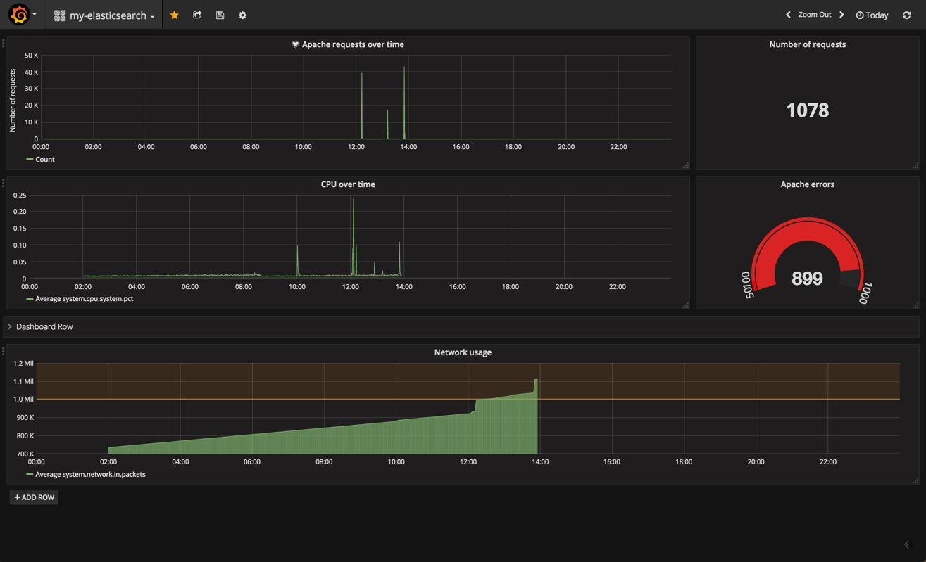
You can create a series of visualizations and then combine them into your own Elastic Beanstalk dashboard:

elastic beanstalk dashboard

Endnotes

Elastic Beanstalk helps developers roll apps into production by taking care of the provisioning and configuration of the AWS resources necessary to run them. One aspect that remains a challenge, though, is logging, and that’s where ELK comes into the picture.

Your next step towards building your ELK-based logging system for Elastic Beanstalk would be to figure out how to enhance the logs. Logz.io provides auto-parsing for most log types, but if you’re running your own stack, you will need to apply filters on the Logstash level for removing redundant data and parsing the logs correctly.

Logz.io is an AI-powered log analysis platform that offers the open source ELK Stack as a cloud service with machine learning technology and can be used for log analysis, IT infrastructure and application monitoring, business intelligence, and more. Start your free trial today!

Daniel Berman

Daniel Berman is Product Evangelist at Logz.io. He is passionate about log analytics, big data, cloud, and family and loves running, Liverpool FC, and writing about disruptive tech stuff.

http://logz.io

logzio paging with onpage

Getting notified when something goes wrong in your environment is a basic requirement in any DevOps or IT operations team. Businesses now expect their engineers to be online 24/7 and respond with maximum speed and efficiency.

A growing number of messaging and alerting tools seek to help these teams comply with this demand. As our CEO, Tomer Levy, explained in InfoWorld, the rise of ChatOps is another natural development in this space, further helping to bridge the gap between developers and operations.

Logs are used to trigger alerts in these messaging applications, so DevOps crews can get alerted as soon as a specific log message is logged by a designated process that is running in your environment. If you’re logging with Logz.io, you have the option to use pre-made integrations to get alerted by a wide range of messaging and monitoring tools such as Slack, PagerDuty, and Datadog.

You can also create your own custom integrations using webhooks, and in this post I’d like to show you how by demonstrating an integration with an interesting paging service called OnPage.

OnPage promises to help DevOps teams keep track of each and every alert triggered in your environment by providing a persistent, detailed, and comprehensive alert management platform. OnPage’s mobile apps (iOS/Android) play the role of traditional pagers, allowing managers to distribute alerts to team members and message them. OnPage offers enterprise users a webhook API for full integration with the service, and we will make use of this to integrate with Logz.io’s alerting mechanism.

Let’s get started!

Setting Up the OnPage WebHook API

Our first step involves generating the credentials for accessing the OnPage API — a client ID and a secret key. This is done in the OnPage dedicated webhook application, where you will need to click Register New Incoming Webhook.

onpage incoming webhook

The credentials don’t have an expiration date and time, and you can create as many keys as you want — but it’s probably a best practice to have only one to make it easier for if you would ever need to remove the integration with Logz.io.

Don’t forget to save the new integration. Otherwise, your credentials will not be registered correctly.

onpage webhooks

Creating a New Logz.io Endpoint

Now that we have the required pieces to set up the integration, we’re going to set up a new alert endpoint in Logz.io.

Under the Alerts tab in Logz.io, select the “Alert Endpoints” page and click “Add Endpoint.”

Select “Custom” from the endpoint type drop-down menu.

add a new endpoint

Enter a name and description for the new endpoint and then configure the webhook URL and method as follows:

URL – enter “https://webhook.onpage.com/gw/v1/page”
Method – select the “POST” method
Header – (leave this option empty)
Body – use the following JSON format:

{
 "clientId": "clientId",
 "secretKey": "secretKey",
 "message": {
   "subject": "Alert from Logz.io",
   "body": "This is an alert from Logz.io",
   "recipients": [
     "OnPageId"
   ],
   "priority": "HIGH"
 }
}

A few comments on the above request.

Be sure to validate the JSON before inserting it in the endpoint configuration. Also, the “OnPageId” is the OnPage ID of the recipient — or, in other words, the person to whom you want to send the alert. The ID is created when the recipient signs into his OnPage app on his mobile device (iOS/Android).

After you save the new endpoint, it will be added to the list of endpoints defined in Logz.io:

list of defined endpoints

Creating a New Alert

Now that the integration is all set up, we can now test it with a new log-based alert.

Creating a new alert in Logz.io is done from the “Discover” tab in Kibana. Enter your query in the “Search” field — in this case, I’m looking at an Apache access log that reports a 504 error (type:apache_access AND response:504):

apache log error

Once you’ve narrowed down the type of log message on which you want to be alerted, click the “Create Alert” button. The query is copied to the Alert Creation Wizard, where it can be modified as desired:

create a new alert

On the first page of the wizard, you will need to configure the trigger conditions — or, in other words, select which specific conditions will trigger an alert.

Then, after naming and describing the alert on the following page, all that’s left to do is to select the OnPage endpoint on the third and final page of the wizard:

select onpage endpoint

Once created, and according to the definitions we entered in the alert, Logz.io will trigger an alert if a 504 response is logged from our Apache web server and a page will be sent to the OnPage recipient.

on page alert

Final Notes

Because logs are the ultimate raw indicator of what is taking place under the hood of both your applications and the infrastructure they are running on, using them to trigger alerts is becoming the standard DevOps practice.

There are two main challenges in setting this up — understanding on which log message you want to trigger an alert (learn about how we use machine learning to do just this) and figuring out the best way to receive and manage these alerts. If you’re looking for an alerting or messaging tool, OnPage’s services are definitely worth exploring.

Happy paging!

Daniel Berman

Daniel Berman is Product Evangelist at Logz.io. He is passionate about log analytics, big data, cloud, and family and loves running, Liverpool FC, and writing about disruptive tech stuff.

http://logz.io

grafana elasticsearch

Now, why would I want to do that?

If I’m using ELK, I already have Kibana — and since version 5.x, Timelion is provided out of the box so I can use that for analyzing time-series data, right?

Well, yes and no.

While very similar in terms of what can be done with the data itself within the two tools, the main differences between Kibana and Grafana lie in configuring how the data is displayed. Grafana has richer display features and more options for playing around with how the data is represented within the graphs.

While it takes some time getting accustomed to building graphs in Grafana, especially if you’re coming from Kibana, the data displayed in Grafana dashboards can be read and analyzed more easily.

Here are some instructions on setting up the integration with Elasticsearch and getting started with your first Grafana dashboard.

Installing Grafana

This article assumes you have an ELK Stack up and running already, so the first step is to install Grafana.

The instructions below are for Ubuntu/Debian. If you’re using a different OS, refer to Grafana’s excellent docs here (if you’re using Docker, that’s probably the easiest way to get Grafana up and running).

To do this, first add the following line to your /etc/apt/sources.list file (don’t worry about the version name, keep it as jessie even if you’re using a more recent version:

deb https://packagecloud.io/grafana/stable/debian/ jessie main

Next, add the Package Cloud key so you can install a signed package:

curl https://packagecloud.io/gpg.key | sudo apt-key add -

Update your repos and install Grafana with:

sudo apt-get update && sudo apt-get install grafana

Last but not least, start Grafana:

sudo service grafana-server start

Open your browser at http://:3000 and use admin/admin as the credentials to access Grafana:

access grafana

Connecting to Elasticsearch

Once installed, your next step is to set up the integration with a data source — in our case, Elasticsearch.

Click on the “Add data source” button displayed in your Grafana Home Dashboard, and configure the connection with Elasticsearch.

A few pointers.

You will be required to enter the name of the Elasticsearch index with which you want to integrate. Use this cURL on the host on which Elasticsearch is installed to get a list of all Elasticsearch indices:

curl -XGET 'localhost:9200/_cat/indices?v&pretty'

An example output:

health status index                 uuid                   pri rep docs.count docs.deleted store.size pri.store.size
yellow open   metricbeat-2017.01.23 VPzuOuthQtSxsmo9bEscGw   5   1      12309            0      3.4mb          3.4mb
yellow open   .kibana               nIq0NUcRT1ejxw4-MwHXWg   1   1          2            0     68.2kb         68.2kb

In the HTTP settings section, you will be required to select the type of access to use. Just to clarify, in the direct access, the URL that you provide is accessed directly from the browser whereas in the proxy access, the Grafana backend acts as a proxy and routes requests from the browser to Elasticsearch.

Here are the settings that I used to connect with an Elasticsearch installed on an AWS EC2 instance:

connect elasticsearch to grafana

Click Save & Test. A green success message means that Elasticsearch was connected successfully.

Creating a Grafana Dashboard

For this tutorial, I defined two data sources for two different Elasticsearch indices — one for Apache logs shipped using Filebeat and the other for server performance metrics to Elasticsearch using Metricbeat.

We’ll start by creating a new dashboard. This is done by clicking on the Grafana icon in the top-left corner and selecting Dashboards → New.

grafana menu

In Grafana 4.1, you have the selection of different visualizations — or “panels,” as they are called in Grafana — to choose from at the top of the dashboard.

We’re going to select the Graph panel, which is the most frequently-used panel type. By default, a nice panel is displayed showing some sort of data over time. Don’t get too excited — this is not your Elasticsearch data but some fake data source Grafana that is using to help us get started.

To edit the graph, you need to click the panel title and then Edit.

edit grafana chart

Our graph is opened in edit mode, with the Metrics tab open. This tab is the most important one because it defines what data to display. Of course, and like in Kibana, the options on display here will vary based on the data source and data type.

Start by removing the fake data source and adding your Elasticsearch data source.

Then click + Add query.

define grafana query

The options for defining what and how the data is to be cut is similar to Kibana — in the query field, define your Lucene query and then select an aggregation type for both the Y (metric) and X (Group by) axes.

In the other tabs, the richness in display options comes to the fore.

In the “General” tab, you define the title and description for the panel. You can also add dynamic links to the panel that can link to other dashboards or URLs.

In the “Axes” tab you can play around with the units and scales for the X and Y axes and add custom labels for each axis.

We can continue to build our panels in a similar way. Grafana has three main panel types on offer — which is a bit limiting, compared to Kibana — but you will find that the three main types (graph, table, single stat) cover most of your monitoring needs.

In no time, you can have a dashboard up and running. Here is an example of an Apache and server performance monitoring dashboard using the two Elasticsearch indices as data sources. Of course, you could hook in any other data source that is supported by Grafana to create a more comprehensive dashboard:

grafana elk dashboard

Summary

From a functionality perspective, it’s hard to point out a critical parity between the two tools. So, if you’ve got your own ELK up and running, there may be no pressing need of abandoning Kibana.

Still, Grafana is well worth exploring for two main reasons. First, it’s extremely easy to set up. It took me just a matter of minutes to get the integration up and running. Second, from a mere usability perspective, Grafana has a much nicer UI and UX.

There are some compatibility issues with integrating Elasticsearch 5.x that you should be aware of — alerting, one of Grafana’s more recent features — does not seem to work well, for example.

If you’re interested in a more detailed comparison between these two great visualization tools, I recommend reading both our high-level comparison and this more technical breakdown by the folks at Rittman Mead.

Daniel Berman

Daniel Berman is Product Evangelist at Logz.io. He is passionate about log analytics, big data, cloud, and family and loves running, Liverpool FC, and writing about disruptive tech stuff.

http://logz.io

machine learning log analytics

Opening a Kibana dashboard at any given time reveals a simple and probably overstated truth — there are simply too many logs for a human to process. Sure, you can do it the hard way, debugging issues in production by querying and searching among the millions of log messages in your system.

But this is far from being a methodological and productive method.

Kibana searches, visualizations, and dashboards are very effective ways to analyze a system, but a serious limitation of any log analytics platform, including the ELK Stack, is the fact that the people running them only know what they know. A Kibana search, for example, is limited to the knowledge of the operator who formulated it.

“Alexa/Cortana/Siri, What’s Wrong With My Production Environment?”

Asking a virtual personal assistant for help in debugging a production system may seem like a far fetched idea, but the notion of using a machine learning approach is actually very feasible and practical.

Machine learning algorithms have proven very useful in recent years at solving complex problems in many fields. From computer vision to autonomous cars to spam filters to medical diagnosis, machine learning algorithms are providing solutions to problems and solving issues where once expert humans were required.

Supervised Machine Learning

Among the various approaches to machine learning, supervised machine learning stands out as one of the most powerful tools in the data scientist’s toolbox.

Supervised machine learning is based on the idea of learning by example. The algorithm is fed with data that relates to the problem domain and meta data that attributes a label to the data. For example, the domain-specific data may be an image, essentially a set of pixels, and a label. This label may indicate that the set of pixels forms a car, a pedestrian, or an important traffic landmark. The process of assigning labels to data is referred to as “labeling,” and it plays a crucial part of obtaining good results from supervised machine learning.

Formulating the problem in this fashion enables machine learning algorithms to sift through huge amounts of data, making the necessary correlations and deducing the interdependencies between the data points.

Dealing with terabytes of log data, we at Logz.io pose this classification question: “Is this log interesting?”

An Ill-Posed Question

The question of log relevancy is not a trivial one. A log entry may prove very useful to one user and completely irrelevant to another. Moreover, in the process of data labeling, interesting logs may not get labeled correctly or at all because they were lost in the clutter.

To tackle the problem of data labeling, we at Logz.io are using the below methodologies:

Use implicit and explicit user behavior.
We pay attention to the ways that our clients interact with our tools. Creating an alert, viewing a log, creating dashboards and other actions are all actions during which our users indicate what is important to them.
Inter-user similarities.
All of our clients are unique, and we cherish every one of them. Our moms’ reassurances notwithstanding, we are also all very similar and use the same components and, therefore, share similar log entries. Consequently, similar users may draw benefits from common labeling.
Harvest public resources such as CQA (community questions and answers) sites and others.
Sites such as Stack Overflow, GitHub, and even Wikipedia contain wealths of information and host a vast pools of knowledge that can be used to evaluate the importance of logs and even propose solutions to the root problems that are indicated by these logs.

Combining data from these resources enables us at Logz.io to create a very rich dataset of labeled logs, together with meta data on the log relevance, frequency and, in some cases, information that shows how to solve the underlying issue.

Training Your Classifier

Once the necessary data — log entries and corresponding labels — has been accumulated, it is possible to construct a log classifier.

Classification can be performed in many ways, and one such method is Linear Support Vector Machines (SVM). This type of classifier offers simple training and is easy to interpret by domain experts.

More information on SVM and its application to text classification can be found here:

For this example, a feature vector needs to be constructed. Using short n-grams usually yields a feature space of a dimension of about 1M dimensions, which is feasible and rich enough to give good results.

Examples of such n-grams and corresponding weight coefficients are presented below. As can be seen, it is very easy to interpret the results and verify them for sanity. Positive values indicate some sort of system failure, whereas negative values indicate a log entry that does not contain an actionable, relevant, state.

unable: 0.671539714688
topic: 0.678756599452
error: 0.788508324168
connected: -0.157199772246
to provider: -0.15319903564
connected successfully: -0.15319903564

Another possibility for training a classifier is to use Random Forests, which are very useful in cases where the features are categorical (non-numerical) and do not fit linear models very well. More information about using Random Forests for classification can be found here:

https://www.stat.berkeley.edu/~breiman/RandomForests/cc_home.htm

While seemingly trivial, this process is very powerful. It may not take a rocket scientist to tell you that “error” is a phrase that may indicate a production issue, but it is virtually impossible for even the best DevOps group in existence to find the correlations and relations between a million phrases that occur in log data. The process of feeding these vast amounts of data to supervised ML algorithms enables the machine to learn from the accumulated knowledge of hundreds of DevOps teams and hundreds of thousands of contributors to knowledge sites.

At Logz.io, we use a set of machine learning algorithms that are able to collect bits and pieces of data — mostly on what users care about in their log data — and fuse all of them together into a supervised process that trains our machine learning code. One of the most powerful parts of the Logz.io learning system is that it learns from the way in which users react to these highlighted events, enabling ongoing supervision and continuous learning.

Integration

Once the classifier was trained, it was integrated into the Logz.io pipeline. We used tools including Spark and Hadoop to run the classifier and machine learning at the scale that was required. The logs that pass the entire classification stage are labeled as “Cognitive Insights” and additional information that has been gathered in the labeling stage is attached to them. This enables Logz.io not only to highlight relevant logs to our customers but also to enrich the logs with additional information.

A Classification Example

Obviously, the Logz.io learning technology is much more complicated and includes a multi-vector analysis, but we thought to share a simplified example. The following log was analyzed in our system (note that specific values have been obfuscated):

“Address <strong>IP_OCTET</strong> maps to <strong>URL</strong>, but this does not map back to the address - POSSIBLE BREAK-IN ATTEMPT!”

The log level for this log was not high, it did not contain any of the usual, trivial, error phrases (“error”, ”fatal”, “exception”, etc’), but it was classified as interesting.

The log was then passed through the augmentation module, and several relevant threads on knowledge sites were found:

These online resources indicate that contrary to the log text, it is more likely to be a DNS issue than an actual security threat.

The system then displays the log and the data to the user in an informative way:

machine learning log analysis

Summary

Utilizing a machine learning approach to log analytics is a very promising way to make life easier for DevOps engineers. Classifying relevant and important logs using supervised machine learning is just the first step to harnessing the power of the crowd and Big Data in log analytics. Adaptive log clustering, log recommendation, and some other cool features are coming soon, so stay tuned!

Logz.io is an AI-powered log analysis platform that offers the open source ELK Stack as a cloud service with machine learning technology. Learn more about our Cognitive Insights technology or create a free demo account to test drive the entire platform for yourself.

athena vs bigquery

The trend of moving to serverless is going strong, and both Google BigQuery and AWS Athena are proof of that. Both platforms aim to solve many of the same challenges such as managing and querying large data repositories.

Announced in 2012, Google describes BigQuery as a “fully managed, petabyte scale, low-cost analytics data warehouse.” You can load your data from Google Cloud Storage or Google Cloud Datastore or stream it from outside the cloud and use BigQuery to run real-time analysis of your data.

In comparison, Amazon Athena, which was released only recently at the 2016 AWS re:Invent conference, is described as an “interactive querying service” that makes it easy to analyze data stored on Amazon S3 using standard SQL-run ad-hoc queries.

In this post, we will show you how you can use both tools and discuss the differences between them such as cost and performance.

User Experience

Executing Queries Using BigQuery

BigQuery can be used via its Web UI or SDK. In this section, we will briefly explain the terms used in the BigQuery service and discuss how you can quickly load data and execute queries.

Before you begin, you will need to go on the Google Cloud Platform to create the project.

project page on google cloud

After creating a new project (BigQuery API is enabled by default for new projects), you can go to the BigQuery page page.

BigQuery allows querying tables that are native (in Google cloud) or external (outside) as well as logical views. Users can load data into BigQuery storage using batch loads or via stream and define the jobs to load, export, query, or copy data. The data formats that can be loaded into BigQuery are CSV, JSON, Avro, and Cloud Datastore backups.

bigquery welcome page

In our demo, we used a simple public dataset and general data that can be used by anyone such as that of Major League Baseball (nice!).

We can click the Compose Query red button to enter the query we want to execute against the desired table. In our case, we looked to display 5,000 rows from the Wikipedia public dataset bigquery-public-data:samples.

We ran the query:

SELECT * FROM [bigquery-public-data:samples.wikipedia] LIMIT 5000;

and got the results in the table as shown below.

Note that BigQuery returned the results in 2.3 seconds, scanning over 35.7 GB of data. Different types of aggregations can be executed, for example, to sum the number of characters to return the lengths of articles.

The List of 5,000 Rows, From the Wikipedia Dataset

The aggregation shown below was completed in 2 seconds, scanning over 2.34 GB of data.

The Sum of the Number of Characters Column in the Wikipedia Table

In addition to the Web UI and command line, users can also connect to BigQuery using ODBC and JDBC drivers to enable it to be used locally with popular SQL tools such as SQL Workbench.

Executing Queries Using Amazon Athena

AWS Athena is based on the Hive metastore and Presto, where the Athena syntax is comprised of ANSI SQL for queries and relational operations such as select and join as well as Hive QL DLL statements for altering the metadata such as create or alter.

Like BigQuery, Athena supports access using JDBC drivers, where tools like SQL Workbench can be used to query Amazon S3. The data formats that can be loaded in S3 and used by Athena are CSV, TSV, Parquet Serde, ORC, JSON, Apache web server logs, and customer delimiters. Compressed formats like Snappy, Zlib, and GZIP can also be loaded.

Amazon Athena’s Web UI is similar to BigQuery when it comes to defining the dataset and tables. Through the Getting Started with Athena page, you can start using sample data and learn how the interactive querying tool works.

As shown below, you can access Athena using the AWS Management Console. In our case, we chose to query ELB logs:

aws athena home page

Let’s try a few queries to see how quickly the results are returned. The queries and results are displayed below the Query Editor window.

The Results from 5,000 Rows of the ELB Logs – 4.73 seconds

The Sum by Request Processing Time Column – 8.78 seconds

Athena vs. BigQuery

In the following sections, we will provide an in-depth comparison of these two tools.

Data Sources

As mentioned above, BigQuery supports native tables. These are optimized for reading data because they are backed by BigQuery storage, which automatically structures, compresses, encrypts, and protects the data. In addition, BigQuery can also run on external storage. In comparison, Athena only supports Amazon S3, which means that a query can be executed only on files stored in an S3 bucket.

Price

The price models for both solutions are the same. Users pay for the S3 storage and the queries that are executed using Athena. AWS Athena is paid per query, where $5 is invoiced for every TB of data that is scanned. Check Amazon’s Athena pricing page to learn more and see several examples.

Google also charges by the amount of data scanned, and the price is the same as for Athena. The storage is $0.02 per GB, which is more or less the same in AWS (the price tiers depends on the overall amount stored). All other operations such as loading data, export, copy or metadata are free.

Performance

When it comes to speed, the native tables in BigQuery show good performance. Below, we examined another public data set called bigquery-public-data.github_repos.licenses. We loaded the same data set to an S3 bucket and executed the following SQL statement, counting the number of licenses in the table (grouped by the license number):

SELECT
   license,
   COUNT(*) AS licenses
FROM
   [bigquery-public-data.github_repos.licenses]
GROUP BY
   license
ORDER BY
   licenses DESC

BigQuery Result for Counting the Licenses – 1.7 seconds

We checked the same results in Athena. The results are shown below:

Athena Result for Counting Licenses – 7.05 seconds

We see that using BigQuery shows better performance than AWS Athena, but obviously that will not always be the case.

It’s important to note that Amazon Athena supports data partition by any key (unlike BigQuery, which supports date only). With Athena, you can also restrict the amount of scanned data by each query — which leads to improved performance and reduced costs.

UDF Support

The next way in which BigQuery and Athena differ are in the User Defined Functions (UDF). In BigQuery, this is a JavaScript function that can be called as part of a query, an action that provides powerful functionality where mixing SQL and the code is possible. One example of this is implementing custom converters that don’t exist, such as the URL decode function.

For data engineers, UDF is a powerful tool that Athena currently does not support, and the only way to add it is to contact their team at at athena-feedback (at) amazon.com. But as we know from Amazon’s release cadence, UDF will be introduced soon.

Summary

So, what can we expect from Athena and BigQuery going forward? At this stage, Athena offers a high-level service for querying data already stored in S3. If you’re already an AWS services user and you have data to analyze, just create a table point on S3 and you’re ready to query. What would be nice to have from Athena is additional operations in a table such as appending results of a query to an existing table.

Overall, Athena as a new product has potential, and it’s worth waiting to see what it will offer in the near future. As far as BigQuery, although some features are missing such as partitioning with any column in a table, the solution is mature and feature-rich, and offers users a good and robust data warehouse solution.

Logz.io is another DevOps tool that is an AI-powered log analysis platform that offers the open source ELK Stack as a cloud service with machine learning technology and can be used for log analysis, IT infrastructure and application monitoring, business intelligence, and more. Start your free trial today!

The AI-powered platform is core to RAC’s digital transformation strategy

TEL AVIV, ISRAEL and BOSTON, MA — Rent-A-Center (RAC), the leading furniture and electronics rent-to-own company, has placed Cognitive Insights, Logz.io’s revolutionary AI-powered IT analytics platform, at the core of its digital transformation strategy.

Cognitive Insights uses machine learning to analyze human interaction with log data to uncover irregularities in IT environments. After embarking on this new system, RAC reported that Cognitive Insights helped the company to properly detect potential threats before they impact customers.

As RAC began its digital transformation, the use of the open source ELK Stack was the obvious software to choose to centralize and monitor log data. The platform removes the necessity for developers and engineers to log directly into the production systems to view log data.

However, RAC found that managing the ELK deployment for performance and reliability turned out to take too much time because the company lacked a dedicated team to maintain the platform. As a result, competing priorities made it impossible to manage, resulting in system instability and various components having out-of-date versions. Most concerning of all, the company found that it was unable to devote the necessary time to the stack until after an incident had already occurred.

To combat these issues, RAC turned to the Logz.io AI-powered log analysis platform that offers the ELK Stack as a enterprise-grade cloud service with machine learning technology. Logz.io’s system includes visualizations, dashboards, and alerts that can be used to better understand Big Data.

Logz.io’s Cognitive Insights, which uses artificial intelligence and machine learning algorithms to analyze how people are interacting with log data, proved itself to be extremely valuable as it alerted the RAC team to multiple failed root login attempts that Rent-A-Center previously had not detected. Though these attempts later turned out to be a routine scan, it left RAC’s security team confident that Cognitive Insights would be able to catch other irregularities of greater consequence in the future.

“Cognitive Insights gave us the confidence that we will be able to detect future anomalies with Logz.io,” says Troy Washburn, Senior DevOps Manager of RAC.

Since employing Logz.io, RAC developers have gained greater visibility and transparency into how their machines and applications are functioning in all environments up through production. Furthermore, they are able to work more quickly and more productively, enabling them to respond to issues more rapidly than ever. In essence, RAC has successfully evolved into a more agile environment with the help of Logz.io’s log analysis platform.

About Logz.io

Logz.io is an AI-powered log analysis platform that offers the world’s most popular logging software, the open source ELK Stack, as an enterprise-grade cloud service with machine learning technology. Visit the the company’s blog on DevOps, log analysis, and ELK and follow Logz.io on Twitter, Facebook, LinkedIn, and Google+.

upgrade elasticsearch 5

We at Logz.io provide the ELK Stack as an end-to-end service on the cloud, so we are always committed to providing the latest and greatest version of the stack.

As soon as Elasticsearch 5 was released back in October, we pushed the upgrading of our existing Elasticsearch 2 clusters to the top of our priority list. In this post, I’ll outline how we performed the upgrade, together with some tips that we learned the hard way.

Why Upgrade in the First Place?

There is a long list of new and improved features in Elasticsearch 5 (see our post on the entire ELK Stack 5.0 as well as Kibana 5 in particular), but the main reason we wanted to perform the upgrade as soon as possible was for the new version’s easier management and maintenance of large-scale clusters.

Two examples of the improvements:

A rollover index. This new feature allows you to define the conditions during which the index will automatically perform a rollover — such as the numbers and ages of documents
A way to limit the total number of mapping fields. A new dynamic index setting allows you to restrict the amount of mapping fields in a cluster instead of having to use an internal account management service

Things to Consider Before Upgrading

New and improved features notwithstanding, there are some issues that we recommend fully understanding before you decide to go ahead with the upgrade process (see Elasticsearch’s documentation for a full list of breaking changes).

There is no rollback. You cannot revert from Elasticsearch 5.x back to version 2.x. So, you should backup your data using snapshots or any other solution before you upgrade to Elasticsearch 5. Also, we recommend that you create a testing cluster to validate that your system continues to work as expected after the upgrade.
Marvel. If you are using the Marvel plugin to monitor your ELK Stack, you should know that it doesn’t exist anymore. In version 5, Marvel was merged into Elastic’s X-Pack, and most of its features are not included in the free Basic subscription. Marvel’s replacement is within the X-Pack’s Monitoring cluster of features.
SDKs. Not all of Elasticsearch’s SDKs are compatible with Elasticsearch 5. This is a major disadvantage right now, but it will probably be resolved soon.
Open-source plugins. Elasticsearch 5 is fairly new, therefore not all the open source plugins are compatible with the latest version. You should check each of them before you decide to upgrade.

How We Upgraded Our Environment with Minimum Downtime

Elastic’s documentation details upgrade instructions here, but our setup required a more specific and customized approach.

Our infrastructure is based entirely on Amazon Web Services and is managed using a set of tools including Puppet with the ec2tagfacts and the puppet-elasticsearch modules. To orchestrate the upgrade, we wrote an Ansible playbook to modify the instance’s AWS tags and then perform the full cluster restart and run Puppet again.

This process involves a certain downtime, so it goes without saying that we tested it internally and extensively before finally executing the upgrade at a time that would guarantee the least disruption.

It’s worth mentioning that we also developed some capabilities in our infrastructure that would help to mitigate downtime for most uses of our log analytics platform, and we will share them in the future.

The order in which we performed the upgrade was as follows:

Master nodes. To allow all the other nodes to connect to the cluster, you should start the master nodes first.
Coordinating nodes. The coordinating nodes are used to coordinate the work for the data nodes, therefore you should start them before the data nodes.
Data nodes. The data nodes are those that actually hold the data, so you should leave them for last — if something did not work in the previous steps, you can skip the upgrade and create new master and coordinating nodes in version 2. Elasticsearch data node upgrades are dependent on the prior two upgrade steps to work. Another advantage is that most of the time spent on recovering the cluster will be spent on the data nodes.

Learn From Our Mistakes

Experience is everything, so here are two tips that we’re happy to share based on what we have learned:

Remove older Java versions to make sure that you are using the latest version as required without having to change the default Java in the instance.
One of the crucial changes in Elasticsearch 5 is that index default settings cannot be configured in the elasticsearch.yml configuration file. It’s crucial to apply all index settings in an order 0 template, but because the template is applied only on the indices that will be created in the future, it is important to apply the same settings to all of the old indices (using the /_settings endpoint) as well. And don’t forget about the new index settings that were introduced in version 5!

In Conclusion

The downside of using the latest technology is that you are more prone to encounter bugs. But with the help of the open source community — of which we are a proud member — we have managed to overcome most of the obstacles.

We expected the Elasticsearch upgrade process for our entire production environment to take much more time than it actually did, and we can attribute that to good preparation and the talented team of people who executed the process.

A final tip: If you do decide to upgrade to Elasticsearch 5, first run it for a while in a non-production environment. This will verify that the deprecated features and breaking changes in the new version will not take down your operation post-upgrade.

Good luck!

upgrade elasticsearch 5

We at Logz.io provide the ELK Stack as an end-to-end service on the cloud, so we are always committed to providing the latest and greatest version of the stack.

Why Upgrade in the First Place?

Two examples of the improvements:

A rollover index. This new feature allows you to define the conditions during which the index will automatically perform a rollover — such as the numbers and ages of documents
A way to limit the total number of mapping fields. A new dynamic index setting allows you to restrict the amount of mapping fields in a cluster instead of having to use an internal account management service

Things to Consider Before Upgrading

There is no rollback. You cannot revert from Elasticsearch 5.x back to version 2.x. So, you should backup your data using snapshots or any other solution before you upgrade to Elasticsearch 5. Also, we recommend that you create a testing cluster to validate that your system continues to work as expected after the upgrade.
Marvel. If you are using the Marvel plugin to monitor your ELK Stack, you should know that it doesn’t exist anymore. In version 5, Marvel was merged into Elastic’s X-Pack, and most of its features are not included in the free Basic subscription. Marvel’s replacement is within the X-Pack’s Monitoring cluster of features.
SDKs. Not all of Elasticsearch’s SDKs are compatible with Elasticsearch 5. This is a major disadvantage right now, but it will probably be resolved soon.
Open-source plugins. Elasticsearch 5 is fairly new, therefore not all the open source plugins are compatible with the latest version. You should check each of them before you decide to upgrade.

How We Upgraded Our Environment with Minimum Downtime

Elastic’s documentation details upgrade instructions here, but our setup required a more specific and customized approach.

The order in which we performed the upgrade was as follows:

Master nodes. To allow all the other nodes to connect to the cluster, you should start the master nodes first.
Coordinating nodes. The coordinating nodes are used to coordinate the work for the data nodes, therefore you should start them before the data nodes.
Data nodes. The data nodes are those that actually hold the data, so you should leave them for last — if something did not work in the previous steps, you can skip the upgrade and create new master and coordinating nodes in version 2. Elasticsearch data node upgrades are dependent on the prior two upgrade steps to work. Another advantage is that most of the time spent on recovering the cluster will be spent on the data nodes.

Learn From Our Mistakes

Experience is everything, so here are two tips that we’re happy to share based on what we have learned:

Remove older Java versions to make sure that you are using the latest version as required without having to change the default Java in the instance.
One of the crucial changes in Elasticsearch 5 is that index default settings cannot be configured in the elasticsearch.yml configuration file. It’s crucial to apply all index settings in an order 0 template, but because the template is applied only on the indices that will be created in the future, it is important to apply the same settings to all of the old indices (using the /_settings endpoint) as well. And don’t forget about the new index settings that were introduced in version 5!

In Conclusion

Good luck!

grafana elasticsearch

Now, why would I want to do that?

If I’m using ELK, I already have Kibana — and since version 5.x, Timelion is provided out of the box so I can use that for analyzing time-series data, right?

Well, yes and no.

While it takes some time getting accustomed to building graphs in Grafana, especially if you’re coming from Kibana, the data displayed in Grafana dashboards can be read and analyzed more easily.

Here are some instructions on setting up the integration with Elasticsearch and getting started with your first Grafana dashboard.

Installing Grafana

This article assumes you have an ELK Stack up and running already, so the first step is to install Grafana.

To do this, first add the following line to your /etc/apt/sources.list file (don’t worry about the version name, keep it as jessie even if you’re using a more recent version:

deb https://packagecloud.io/grafana/stable/debian/ jessie main

Next, add the Package Cloud key so you can install a signed package:

curl https://packagecloud.io/gpg.key | sudo apt-key add -

Update your repos and install Grafana with:

sudo apt-get update && sudo apt-get install grafana

Last but not least, start Grafana:

sudo service grafana-server start

Open your browser at http://:3000 and use admin/admin as the credentials to access Grafana:

access grafana

Connecting to Elasticsearch

Once installed, your next step is to set up the integration with a data source — in our case, Elasticsearch.

Click on the “Add data source” button displayed in your Grafana Home Dashboard, and configure the connection with Elasticsearch.

A few pointers.

curl -XGET 'localhost:9200/_cat/indices?v&pretty'

An example output:

health status index                 uuid                   pri rep docs.count docs.deleted store.size pri.store.size
yellow open   metricbeat-2017.01.23 VPzuOuthQtSxsmo9bEscGw   5   1      12309            0      3.4mb          3.4mb
yellow open   .kibana               nIq0NUcRT1ejxw4-MwHXWg   1   1          2            0     68.2kb         68.2kb

Here are the settings that I used to connect with an Elasticsearch installed on an AWS EC2 instance:

connect elasticsearch to grafana

Click Save & Test. A green success message means that Elasticsearch was connected successfully.

Creating a Grafana Dashboard

We’ll start by creating a new dashboard. This is done by clicking on the Grafana icon in the top-left corner and selecting Dashboards → New.

grafana menu

In Grafana 4.1, you have the selection of different visualizations — or “panels,” as they are called in Grafana — to choose from at the top of the dashboard.

To edit the graph, you need to click the panel title and then Edit.

edit grafana chart

Start by removing the fake data source and adding your Elasticsearch data source.

Then click + Add query.

define grafana query

In the other tabs, the richness in display options comes to the fore.

In the “General” tab, you define the title and description for the panel. You can also add dynamic links to the panel that can link to other dashboards or URLs.

In the “Axes” tab you can play around with the units and scales for the X and Y axes and add custom labels for each axis.

grafana elk dashboard

Summary

There are some compatibility issues with integrating Elasticsearch 5.x that you should be aware of — alerting, one of Grafana’s more recent features — does not seem to work well, for example.

aws x-ray

Back at AWS re:Invent in November, one could not help but feel overwhelmed by the amount — and the potential impact — of the new features and services announced. I covered some of these new features in this blog post, but one announcement I missed out on was Amazon X-Ray.

X-Ray, as it’s name implies, allows you to get visibility into the performance of your deployed applications by providing traces of requests as they are routed through the different service waypoints. It can thus be used to not only monitor the performance of the requests but also to identify bottlenecks and errors.

X-Ray works by adding HTTP headers to each request and passing on those headers to request handlers. At each waypoint, data “segments” are collected and then later aggregated into individual traces.

The service is currently in preview mode and supports only .NET, Java, and Node.js apps running on EC2, ECS, Elastic Beanstalk, and API Gateway, and the X-Ray SDK captures metadata for a variety of databases.

Let’s take a closer look.

Getting Started

Since X-Ray is in preview mode, you have to sign up first.

Once you’re given access, head over to the X-Ray console, where you will be presented with two ways to get started:

getting started with aws x-ray

You can use your own application, and if that’s the path you’re interested in taking, you’re going to want to check out the documentation on the various available SDKs for Java, Node.js, and .NET applications.

However, the easiest and fastest way to get acquainted with X-Ray — and also the one used for the purposes of writing this post — is using the supplied Node.js demo application.

At the end of the detailed steps, you will have an Express (Node.js) app deployed on Elastic Beanstalk that serves a simple signup service that stores data on AWS DynamoDB and uses AWS SNS to send notifications.

aws x-ray sample application

Next, start generating requests! As specified in the app, hitting the Start button will generate up to ten signup requests per minute with a duplicate signup each minute.

After a while, stop the requests and open the Service Map tab in the console. As you can see, it now starts to get interesting:

map of aws requests

What you see is a nice map of all the requests routed between the different AWS service endpoints. In the case of the demo app, we can see requests coming from the client, to EC2, and then on to DynamoDB and SNS.

As you can see, the folks at AWS made sure our data contains some warnings. Opening the legend on the right gives us insight into the meanings of the different colors:

aws request map

Each of the nodes in the map represents a request waypoint, and behind them are tracked traces. Clicking any of the nodes will lead you to these traces:

aws x-ray traces

Note the Filter field at the top of the console — this field allows you to search traces using a simple filtering syntax. You can build your own custom filter or use the provided filters.

For example, say we want to narrow down the list of service requests to only those with errors:

service("xray-demo.htuaqjkx9a.us-east-1.elasticbeanstalk.com") {error = true}

aws service request error log

We can see that POST requests originating from the signup page are triggering 409 errors. To troubleshoot the root cause, we’re going to open one of the available traces:

available traces

What we see is a timeline of the request — and we can see that calls to DynamoDB are failing, for some reason.

Clicking on the DynamoDB segment provides us with additional insight — we can see that the request to DynamoDB is resulting in a 400 response:

dynamo db traces

Taking a look at the DynamoDB subsegment traced by X-Ray, we can see that a ‘ConditionalCheckExceptionFailed’ exception was triggered by the request:

dynamoDB subsegment traced by x-ray

Summary

With the growing adoption of microservices and as IT as a whole becomes more distributed, the case for distributed stack tracing for application performance monitoring is obvious. The ability to trace requests from clients to the various the services running behind the scenes is crucial to be able to troubleshoot issues and identify bottlenecks in real-time.

AWS did not invent the wheel in this case — there are some big players in the space that do an exceptionally good job at APM and stack tracing. Being only a preview, X-Ray still has some way to go before it can take on these players.

The ability to seamlessly access logs for the services represented in the Service Map is one missing feature, for example, as is support for other languages and frameworks. But X-Ray is indeed huge news for DevOps crews building their apps on AWS, and there is little doubt AWS will make sure the folks at New Relic start sweating.

february 2017 product updates

It’s great starting the new year with product announcements and the past month has seen a number of new features and updates that we thought you would like to hear about. Below is a short recap of the main updates.

As always, kudos to our development team for an awesome job!

Search API

The Logz.io Search API allows our users to safely and securely query the data they are shipping to Logz.io using the Elasticsearch query DSL. Replacing the older Query API, the new API can be used for integration with third-party platforms and compliments the Logz.io Kibana-based UI.

For examples and more information, check out this blog post.

Sub Accounts

We’re happy to announce that we’ve added the ability to run sub-accounts under one single main account, enabling more efficient account control and management:

logzio subaccounts

Under one main-account, different environments can be defined, each with its own access token and its own group of users. Different data volumes and retention periods can be defined per sub-account. For example, under a main account, a manager could define one sub-account for development, one for staging and another for production.

Cognitive Insights Updates

Cognitive Insights, the AI-based technology added on top of the ELK Stack for pointing out logs that really matter, has been revamped with new functionality and a new look and feel and better UX.

Users can now create an alert for a specific insight, assign an insight to another user, customize the insight by editing its description and severity level and more:

New Java and .NET Log Shippers

New log shippers have been introduced for log4j1, log4j2, and Java core — all based on an innovative queuing mechanism that ensures persistency in case of network outages.

We’ve also added new shippers for log4net and nlog, making it easier to send logs from .NET applications.

Datadog, PagerDuty and BigPanda Integrations

New pre-made integrations have been added to the Logz.io alerting feature, making it extremely easy to send alerts via some of the most popular DevOps alerting and messaging applications.

Using these end-points, Logz.io users can now send log-based alerts to Datadog, PagerDuty and BigPanda.

alert endpoints

We have some more great features on the way, so stay tuned!

monitoring dockerized elk stack

The ELK Stack is today the world’s most popular log analysis platform. It’s true.

Trump and humor aside — and as we’ve made the case in previous posts — running an ELK Stack in production is not a simple task, to say the least, and it involves numerous challenges that consume both time and resources. One of these challenges involves monitoring the stack — understanding when your Elasticsearch cluster is stretched to the limit and when your Logstash instances are about to crash.

That’s why if you’re running ELK on Docker, as many DevOps team are beginning to do, it’s imperative to keep tabs on your containers. There are plenty of monitoring tools out there, some specialized for Dockerized environments, but most can get a bit pricey and complicated to use as you go beyond the basic setup.

This article explores an alternative, easy and open source method to monitor a Dockerized ELK: Using Prometheus as the time-series data collection layer and Grafana as the visualization layer.

Prometheus has an interesting story. Like many open source projects, it was initially developed in-house by the folks at SoundCloud, who were looking for a system that had an easy querying language, was based on a multi-dimensional data model, and was easy to operate and scale. Prometheus now has an engaged and vibrant community and a growing ecosystem for integrations with other platforms. I recommend reading more about Prometheus here.

Let’s take a closer look at the results of combining Prometheus with Grafana to monitor ELK containers.

Installing ELK

If you haven’t got an ELK Stack up and running, here are a few Docker commands to help you get set up.

The Dockerized ELK I usually use is: https://github.com/deviantony/docker-elk.

With rich running options and great documentation, it’s probably one of the most popular ELK images used (other than the official images published by Elastic).

Setting it up involves the following command:

git clone https://github.com/deviantony/docker-elk.git

cd docker-elk

sudo docker-compose up -d

You should have three ELK containers up and running with port mapping configured:

CONTAINER ID         IMAGE                     COMMAND                   CREATED              STATUS               PORTS                                            NAMES

9f479f729ed8         dockerelk_kibana          "/docker-entrypoin..."   19 minutes ago   Up 19 minutes        0.0.0.0:5601-&gt;5601/tcp                        dockerelk_kibana_1

33628813e68e         dockerelk_logstash        "/docker-entrypoin..."   19 minutes ago   Up 19 minutes        0.0.0.0:5000-&gt;5000/tcp                        dockerelk_logstash_1

4297ef2539f0         dockerelk_elasticsearch   "/docker-entrypoin..."   19 minutes ago       Up 19 minutes    0.0.0.0:9200-&gt;9200/tcp, 0.0.0.0:9300-&gt;9300/tcp   dockerelk_elasticsearch_1

Don’t forget to set the ‘max_map_count’ value, otherwise Elasticsearch will not run:

sudo sysctl -w vm.max_map_count=262144

Installing Prometheus and Grafana

Next up, we’re going to set up our monitoring stack.

There are a number of pre-made docker-compose configurations to use, but in this case I’m using the one developed by Stefan Prodan: https://github.com/stefanprodan/dockprom

It will set up Prometheus, Grafana, cAdvisor, NodeExporter and alerting with AlertManager.

To deploy, use these commands:

git clone https://github.com/stefanprodan/dockprom

cd dockprom

docker-compose up -d

After changing the Grafana password in the user.config file, open up Grafana at: http://<serverIP>:3000, and use ‘admin’ and your new password to access Grafana.

Defining the Prometheus Datasource

Your next step is to define Prometheus as the data source for your metrics. This is easily done by clicking Creating your first datasource.

The configuration for adding Prometheus in Grafana are as follows:

configuration to add prometheus in grafana

Once added, test and save the new data source.

Adding a Monitoring Dashboard

Now that we have Prometheus and Grafana set up, it’s just a matter of slicing and dicing the metrics to create the beautiful panels and dashboards Grafan is known for.

To hit the ground running, the same GitHub repo used for setting up the monitoring stack also contains some dashboards we can use out-of-the-box.

In Grafana, all we have to do is go to Dashboards -> Import, and then paste the JSON in the required field. Please note that if you changed the name of the data source, you will need to change it within the JSON as well. Otherwise, the dashboard will not load.

The Docker Containers dashboard looks like this:

docker containers dashboard

It really is that simple — in a matter of minutes, you will have a Docker monitoring dashboard in which you will be able to see container metrics on CPU, memory, and network usage.

Another useful dashboard for your Docker environment is the Docker Host dashboard, which is also available in the same repo and uploaded the same way. This dashboard will give you an overview of your server with data on CPU and memory, system load, IO usage, network usage, and more.

docker host dashboard

Pictures are worth a thousand words, are they not?

The flat lines in the screenshots reflect the fact that there is no logging pipeline in action. As soon as we establish a basic pipeline, we can see our Elasticsearch and Logstash containers beginning to pick up.

As you can see in the case below, I’m using logspout to forward syslog logs:

use logsprout to forward syslog logs

This, of course, is just a basic deployment — an Elasticsearch container handling multiple indices and documents will present with more graphs in the “red” — meaning dangerous — zone.

Summary

There are various ways of monitoring the performance of your ELK Stack, regardless of where you’re running it (for example, on Docker).

In a previous post, Roi Ravhon described how we use Grafana and Graphite to monitor our Elasticsearch clusters. Since the release of Elastic Stack 5.x, monitoring capabilities have been built into the stack and even Logstash, the performance bane of the stack, now has a monitoring solution included in X-Pack.

But if you’re using Docker, the combination of Prometheus and Grafana offers an extremely enticing option to explore for reasons of ease of use and functionality.

It’s definitely worth exploring, and if worse comes to worst — sudo docker rm.

dam spillover elk stack

Natural disasters and other types of dramatic events taking place over the globe sometimes provide good opportunities to those interested in practicing their data analysis and visualization pipelines.

These days, publicly available datasets such as the one explored below, can be easily retrieved and from a variety of open repositories, stored in a datastore, and then analyzed with your tool of choice.

This article will show how to ingest the data collected during the recent Oroville Dam incident into the ELK Stack via Logstash and then visualize and analyze the information in Kibana. This same process can be used for virtually any public dataset.

The Oroville Dam data

The California Department of Water Resources publishes rich datasets on all the water sources in the state, so it was extremely easy to query the website for the required data.

As you can see, the query results in a dataset showing the following metrics collected by the sensors deployed at the dam:

Reservoir Elevation
Reservoir Storage
Dam Outflow
Dam Inflow
Spillway Outflow
Rain
Volts

All that is required is to copy the data into a text file so it can be ingested into Elasticsearch via Logstash.

The Logstash configuration

When analyzing logs, parsing and filtering the data during ingestion is a critical step in the pipeline. This process is what helps give the logs the context needed so that they can be later be analyzed more easily in Kibana.

The same rule applies in our case. We want the time-ordered readings from the dam sensors to be parsed correctly so each field is mapped correctly. The way to do this is of course using grok.

A sample measurement is:

02/06/2017 03:00     849.47    2801248   29703     31700     29792     29.68     13.4

So, the configuration for Logstash in our case looks as such:

input {
 file {
       path => "/logs/oroville.log"
       start_position => "beginning"
       type => "log"
   }
}

filter {
 if [type] == "log"  {
   grok {
     match => [
       "message", '%{DATA:timestamp}\t%{DATA:Reservoir_Elevation:int}\t\t%{DATA:Reservoir_Storage:int}\t\t%{DATA:Dam_Outflow:int}\t\t%{DATA:Dam_Inflow:int}\t\t%{DATA:Spillway_Outflow:int}\t\t%{DATA:Rain:int}\t\t%{GREEDYDATA:Volts:int}\t'
     ]
   }
   date {
     match => [ "timestamp" , "MM/dd/yyyy HH:mm" ]
     remove_field => [ "timestamp" ]
     timezone => "PST8PDT"      
   }
 }
}
output {
   tcp {
   host => "listener.logz.io"
   port => 5050
   codec => json_lines
 }
}

We are using the file input plugin to pull the readings, grok filters to parse the message, and the output is pointing to our Logz.io listerners. If you were using your own ELK Stack, you would need to change this to point to your Elasticsearch instance.

Analyzing the data

When you open Kibana, the sensor readings will look as follows:

sensor readings

All the metrics measured from the different sensors at the dam are mapped, so the data is much easier to slice and dice.

Let’s start with visualizing the average amount of rain measured. To do this, we will use a bar chart in which each bar represents a day within the time period analyzed:

average amount of rain

We can see a gradual rise of rainfall (in inches) as the event grew worse.

How about the storage level of the reservoir held back by the dam? In this case, we’re using a line chart visualization to see how the reservoir levels rise over time:

reservoir levels

The max capacity of the reservoir is just under 3.54 million acre-feet, and so we can see how this capacity was surpassed during the crisis. We can also add a traffic light visualization to display the breach:

display breach

The data for the spillover (measured in cubic feet per second) — the emergency drainage mechanism to handle overflows — is a bit more erratic and can be explained by how the event developed, with various tactics applied and failing one after the other:

spillover data

The total amount of water spilled over during the incident and as measured by the dam sensors can be displayed using a Kibana metric visualization:

water amount spilled

Adding all of these into one dashboard gives us a more comprehensive picture of the event:

dashboard

This is just an example of how the ELK Stack can easily be used to ingest and visualize data, but of course, the stack is designed for much larger datasets.

As an endnote, I’d like to express my sympathy with the 200,000 people evacuated from their homes during this event.

Thank you to the State of California for making this data available.

Logz.io helps healthcare IT departments analyze log data to detect anomalies, prevent failures, and protect patient information

TEL AVIV, ISRAEL and BOSTON, MA, February 27, 2017 — Logz.io announced today that the company has become the first open source powered log analytics platform to be HIPAA-compliant. Logz.io offers an AI-powered ELK Stack (Elasticsearch, Logstash, and Kibana) which is the world’s most popular logging platform.

Already SOC 2 and ISO 27001 compliant, a fact that helped the company land top-notch customers such as Dyn, Logz.io’s newest HIPAA certification reveals their commitment to security for health-related organizations. HIPAA (the Health Insurance Portability and Accountability Act of 1996) is a federal U.S. legislation that ensures data privacy and security measures to protect medical information.

In the United States, ensuring that all private health related data is secure is critical for healthcare operations. However, security becomes increasingly difficult to guarantee as organizations implement more and more technologies. HIPAA regulations require that any new technology employed by healthcare organizations comply with its high security standards in order to protect personal health-related information.

As a result of Logz.io’s HIPAA certification, the IT departments of a greater number of healthcare-related organizations will be able to use log data to obtain better insights into their systems and applications, joining the company’s existing healthcare customers such as Stanley Health and Maxwell Health. By using a HIPAA-compliant analytics platform, healthcare IT departments will have the superior capability to detect anomalies, failures, and security breaches that may later affect their patients.

“Becoming HIPAA-compliant was extremely important to us,” says Logz.io Co-founder and CEO Tomer Levy. “Healthcare institutions are undergoing a process of digital transformation through the incorporation of a greater number of technologies and real-time services. Now that Logz.io is HIPAA-compliant, we can help these companies leverage advanced analytics technologies and assist them with their digital transformations.”

With the company’s newly attained HIPAA certification, Logz.io becomes one of the only log analysis platforms that is certified to be used in the healthcare field. As a result, Logz.io can help more hospitals, insurance companies, medical offices, pharmaceutical companies, and other organizations to analyze log data and monitor their IT systems.

About Logz.io

We all like a pretty dashboard. For us data nerds, there’s something extremely enticing about the colors and graphs depicting our environment in real-time. But while Kibana and Grafana bask in glory, there is a lot of heavy lifting being done behind the scenes to actually collect the data.

This heavy lifting is performed by a variety of different tools called log forwarders, aggregators or shippers. These tools handle the tasks of pulling and receiving the data from multiple systems, transforming it into a meaningful set of fields, and eventually streaming the output to a defined destination for storage.

Fluentd is one of the most popular log aggregators used in ELK-based logging pipelines. In fact, it’s so popular, that the “EFK Stack” (Elasticsearch, Fluentd, Kibana) has become an actual thing. A survey by Datadog lists Fluentd as the 8th most used Docker image. Fluent Bit is a relatively new player in town, but is also rising in popularity, especially in Docker and Kubernetes environments.

And so users are now wondering what part Fluent Bit should and can play in a logging pipeline. Is this a new and improved version of Fluentd? Should we retire Fluentd in favor of Fluent Bit? Should the two be used in tandem? In this article, I’ll be providing a high-level comparison so users can understand the difference between the two and when to use them.

What is Fluentd?

Fluentd is an open source log collector, processor, and aggregator that was created back in 2011 by the folks at Treasure Data. Written in Ruby, Fluentd was created to act as a unified logging layer — a one-stop component that can aggregate data from multiple sources, unify the differently formatted data into JSON objects and route it to different output destinations.

Design wise — performance, scalability, and reliability are some of Fluentd’s outstanding features. A vanilla Fluentd deployment will run on ~40MB of memory and is capable of processing above 10,000 events per second. Adding new inputs or outputs is relatively simple and has little effect on performance. Fluentd uses disk or memory for buffering and queuing to handle transmission failures or data overload and supports multiple configuration options to ensure a more resilient data pipeline.

Fluentd has been around for some time now and has developed a rich ecosystem consisting of more than 700 different plugins that extend its functionality. Fluentd is the de-facto standard log aggregator used for logging in Kubernetes and as mentioned above, is one of the widely used Docker images.

If you’re an ELK user, all this sounds somewhat similar to what Logstash has to offer. There are of course some differences, and we cover some of these in this article.

What is Fluent Bit?

Fluent Bit is an open source log collector and processor also created by the folks at Treasure Data in 2015. Written in C, Fluent Bit was created with a specific use case in mind — highly distributed environments where limited capacity and reduced overhead (memory and CPU) are a huge consideration.

To serve this purpose, Fluent Bit was designed for high performance and comes with a super light footprint, running on ~450KB only. An abstracted I/O handler allows asynchronous and event-driven read/write operations. For resiliency and reliability, various configuration option are available for defining retries and the buffer limit.

Fluent Bit is also extensible, but has a smaller eco-system compared to Fluentd. Inputs include syslog, tcp, systemd/journald but also CPU, memory, and disk. Outputs include Elasticsearch, InfluxDB, file and http. For Kubernetes deployments, a dedicated filter plugin will add metadata to log data, such as the pod’s name and namespace, and the containers name/ID.

Comparing Fluentd and Fluent Bit

Both Fluentd and Fluent Bit were developed by Treasure Data to help users build centralized, reliable and efficient logging pipelines. The vision behind Fluentd, and later on, Fluent Bit, was to help overcome some of the challenges involved in logging production environments — formatting unstructured data, aggregation from multiple data sources, resiliency and security.

While there are architectural and design similarities between the two tools, there are also some core differences that should be taken into consideration when picking between the two.

Below is a table summing up the differences between the two tools:

Source: Fluent Bit documentation

Performance

As seen in the table above, while Fluentd can boast efficiency and a relatively small footprint, Fluent Bit takes it up a notch or two. To gauge the difference, take a look at the recommended default specs for running the two tools in Kubernetes. You can do the math yourselves.

Fluentd:

resources:
  limits:
    memory: 500Mi
  requests:
    cpu: 100m
    memory: 200Mi

Fluent Bit:

resources:
  requests:
    cpu: 5m
    memory: 10Mi
  limits:
    cpu: 50m
    memory: 60Mi

In an environment consisting of hundreds of servers, the aggregated effect on CPU and memory utilization is substantial.

Aggregation

Fluent Bit acts as a collector and forwarder and was designed with performance in mind, as described above. Fluentd was designed to handle heavy throughput — aggregating from multiple inputs, processing data and routing to different outputs. Fluent Bit is not as pluggable and flexible as Fluentd, which can be integrated with a much larger amount of input and output sources.

Monitoring

Fluent Bit ships with native support for metric collection from the environment they are deployed on. A variety of input plugins, such as cpu and disk, will collect data on CPU and memory usage, and forward them to a selected output. Version 0.13 also ships with support for Prometheus metrics. Fluentd does not ship with this functionality and would most likely act as the aggregator for these metrics.

Ecosystem

While Fluentd and Fluent Bit are both pluggable by design, with various input, filter and output plugins available, Fluentd (with ~700 plugins) naturally has more plugins than Fluent Bit (with ~45 plugins), functioning as an aggregator in logging pipelines and being the older tool. Fluentd’s history contributed to its adoption and large ecosystem, with the Fluentd Docker driver and Kubernetes Metadata Filter driving adoption in Dockerized and Kubernetes environments.

Community

Taking a look at the code repositories on GitHub provides some insight on how popular and active both these projects are.

Fluentd

Stars: 6423
Forks: 777
Watch: 339
Contributors: 138
Commits: 4165

Fluent Bit

Stars: 586
Forks: 135
Watch: 46
Contributors: 40
Commits: 3173

So, when do I use Fluentd or Fluent Bit?

In a way, Fluent Bit is to Fluentd, what Beats are to Logstash — a lightweight shipper that can be installed as agents on edge hosts or devices in a distributed architecture.

In Kubernetes for example, Fluent Bit would be deployed per node as a daemonset, collecting and forwarding data to a Fluentd instance deployed per cluster and acting as an aggregator — processing the data and routing it to different sources based on tags.

Same goes for an IoT architecture, where Fluent Bit is installed per device, sending data to a Fluentd instance.

Fluent Bit can be used on it own of course but has far less to offer in terms of aggregation capabilities and with a much smaller amount of plugins for integrating with other solutions.

Summing it up

The difference between Fluentd and Fluent Bit can therefore be summed up simply to the difference between log forwarders and log aggregators. The former are installed on edge hosts to receive local events. Once received, the event is forwarded to the log aggregators. The latter are daemons that receive streams of events from the log forwarders, buffer them and periodically upload the data to a data store of some sorts.

The combination of Fluentd and Fluent Bit is becoming extremely popular in Kubernetes deployments because of the way they compliment each other — Fluent Bit acting as a lightweight shipper collecting data from the different nodes in the cluster and forwarding the data to Fluentd for aggregation, processing and routing to any of the supported output destinations.

The rise of Kubernetes will only help drive adoption of Fluent Bit and it would not surprise anyone if the ecosystem around this logging tool explodes with new plugins and features.

Logz.io is an AI-powered log analytics platform that combines advanced machine learning with the open-source ELK Stack. Find out how it can help make log analysis simpler and more insightful!

Learn More!

As an open-source system for automating deployment, scaling, and management of containerized applications, Kubernetes has grown immensely in popularity. Increasingly, we are also beginning to come across platforms offering Kubernetes as both a hosted and managed service.

In this article, we are going to lay out some differences between hosted and self-hosted services and analyze five popular services currently available: Google’s Kubernetes Engine, Azure Kubernetes Service (AKS), Amazon’s Elastic Container Service for Kubernetes (Amazon EKS), and IBM’s Cloud Container Service and Rackspace.

Hosted vs. Self Hosted

Kubernetes is the industry-leading, open-source container orchestration framework. Created by Google and currently maintained by the Cloud Native Computing Foundation (CNCF), it took the container industry by storm thanks to all its experience in handling large clusters. Currently, it is being adopted by enterprises, governments, cloud providers, and vendors thanks to its active community and feature-set.

Self-hosting Kubernetes can be extremely difficult if you do not have the necessary expertise. There are a large number of network, service discovery setups, and Linux configurations on several machines. Moreover, since Kubernetes manages your entire infrastructure, you have to keep it updated to guard against attacks. Beginning with Version 1.8, Kubernetes has provided a tool called kubeadm that allows a user to run Kubernetes on a single machine in order to test it.

On the other hand, if you opt for a hosted, or managed Kubernetes, it doesn’t require that you know a lot or have a great deal of experience with infrastructure. You just need to have a subscription in a cloud provider and it will deploy and keep everything running and updated for you.

When you are ready to scale up to more machines and higher availability, you’ll find that a hosted solution is the easiest to create and maintain and that there is a whole world of possibilities and services to choose from. In the next section, we will talk about the most popular hosted services on the market and analyze them one by one.

Hosted Services

I’ve selected five hosted services and will analyze them separately and compare them with some popular Kubernetes features so you can decide for yourself.

Google’s Cloud Kubernetes Engine

Google’s Kubernetes engine is one of the oldest Kubernetes-hosted services available. Since Google is the original creator of Kubernetes, it is one of the most advanced Kubernetes managers, with a wide array of features available.

Azure Kubernetes Service (AKS)

Azure Kubernetes Service is the Microsoft solution for hosting Kubernetes. The service was recently made available to the general public, but Microsoft previously offered an older version of its managed service called Azure Container Service. With the older service, the user was able to choose between Kubernetes, DC/OS, and Docker Swarm, but it does not have the level of detail available for Kubernetes on its new service.

Amazon’s Elastic Container Service for Kubernetes (Amazon EKS)

Amazon’s EKS is one of the latest services available. Recently, Amazon accepted the challenge of creating its own managed Kubernetes instance instead of a proprietary one. The service is Kubernetes certified and can manage several AWS regions in a single cluster (more details in the next section).

IBM’s Cloud Container Service

IBM’s Cloud Container Service has been available since March 2018, so it is one of the oldest-managed services available on the major clouds. Though not as popular as the three names before, the IBM Cloud is experiencing rapid growth and popularity over enterprise companies.

Rackspace KAAS

Rackspace Kubernetes as a service was launched in June 2018 and still has a lot of the best Kubernetes features as we shall see in the next section. Rackspace is a multi-cloud consulting company and therefore can provide solutions such as multi-cloud portability through many other clouds.

Hosted Services Comparison

In this section, I’ve selected a few Kubernetes characteristics and compare how they are implemented on each hosted service mentioned in the previous section.

Feature \ Service	Google Cloud Kubernetes Engine	Azure Kubernetes Service	Amazon Elastic Container Service for Kubernetes	IBM Cloud Container Service	Rackspace KAAS
Automatic Update	Auto or On-demand	On-demand	N/A	On-Demand	N/A
Load Balancing and Networking	Native	Native	Native	Native	Native
Auto-scaling nodes	Yes	No, but with your own configuration	Yes	No	No
Node-groups	Yes	No	Yes	No	N/A
Multiple Zones and Regions	Yes	No	No	Yes	N/A
RBAC	Yes	Yes	Yes	Yes	Yes
Bare metal nodes	No	No	Yes	Yes	Yes

Automatic Update

To update your cluster version to the latest one you will need to employ automatic updates. Google cloud offers automatic updates, with no manual operation required and Azure and IBM offer on-demand version upgrades. It is not clear how AWS and Rackspace will work since the latest version has been available (v1.10) since its launch.

Load Balancing and Networking

There are two types of load balancing: internal and public services. As its name says, an internal load balancer distributes calls between container instances while the public ones distribute the container instances to the external cluster world.

Native load balancers means that the service will be balanced using own cloud structure and not an internal, software-based, load balancer. Figure 1 shows an Azure Dashboard with a cloud-native load balancer being used by the Kubernetes solution.

Figure 1 – Native load balancer

Auto-scaling

Kubernetes can natively scale container instances to address performance bottlenecks, which is one of its major features and is part of any Kubernetes hosted or self-hosted version. Nevertheless, when it comes to increasing or decreasing the number of nodes (VM’s) running on the cluster depending on the resource utilization, only a few hosted services provide a solution.

The auto-scaling solution provides an easy way to reduce cluster costs when your workload varies during the day. For example, if your application is mostly used during commercial hours, Kubernetes would increase the node count to provide more CPU and memory during peak hours while decreasing to just one node after peak hours. Without autoscaling, you would have to manually change the number of nodes or leave it high (and pay more) to be able to handle peak hours.

Google Cloud provides an easier solution: you can adjust the GUI or the CLI, specify the VM size, and the minimum and maximum number of nodes. Everything else is managed by the provider. Amazon EKS takes second place, it uses AWS’s own autoscaler that can be used for anything on its cloud but it is more difficult to configure compared to Google Cloud. Azure lacks this feature , but a tool called Kubernetes autoscale, provided by Kubernetes itself, gives you everything you need. IBM and Rackspace clouds, unfortunately, do not provide this feature.

Node pools

Node pools are useful Kubernetes features that allow you to have different types of machines in your cluster. For example, a database instance would require faster storage, while a CPU heavy software would not require a faster storage at all.

Once again, Google Cloud already has this feature and Amazon EKS is following their lead. Azure has it on its roadmap and promises it will deliver by the end of the year. Currently there is no information via IBM and Rackspace as to when exactly it will be available.

Multiple zones

Multiple zones allow the cluster to be in more than one region over the world. This allows lower latency per request and, sometimes, reduced costs. The cluster can be configured to direct the nearby node to respond to a request.

Currently, only Google Cloud and IBM cloud provide multiple regional zones.

RBAC

Role-based access control (RBAC) provides a way for admins to dynamically configure policies though Kubernetes’s API. All of the evaluated, hosted services provide RBAC implementations.

Bare metal clusters

Virtual Machines are computers that sit in an emulation layer between the machine and the physical hardware. This highly optimized durable layer, increases computing consumption. Containers are similar to VM when compared in terms of portability and sand-boxing, but they can touch the hardware directly, which is a huge advantage.

Bare metal machines are just the physical hardware for rent. They are quite complex to deploy and payment differs from the VM’s due to the higher operational cost. Currently, only two cloud providers allow cluster nodes to be a bare metal machines: IBM, Rackspace, and AWS.

Conclusion

Kubernetes is a shining new start to the devops area. As such, almost all major cloud providers are in a race to provide better and easier solutions for Kubernetes. Managing Kubernetes itself can be difficult and costly, and any degree of auto-management sufficiently reduces costs and improves reliability.

Using Kubernetes also provides an effective way to avoid vendor-lock-in solutions: since every cloud provider already has its own Kubernetes instance, it is easier to change providers while maintaining all your scripts.

Due to Google’s leadership and involvement with Kubernetes, Google Cloud would be a good option for any new cluster: the majority of features have been available from the beginning and new updates are applied quickly. For larger deployments, try and avoid services that ignore node groups – each image has different requirements that will be better suited in different machines. In the case of CPU-bound processes, such as batch processing or big data analysis, solutions that provides bare metal machines (e.g. IBM and Rackspace) might provide better performance.

Looking to take your DevOps initiatives to the next level? Find out how our customers used Logz.io!

Learn More!

Elasticsearch 6.3 included some major new features, including rollups and Java 10 support, but one of the most intriguing additions in this version is SQL support.

According to DB-Engines, Elasticsearch ranks 8th in popularity, trailing after Oracle, MySQL, PostgreSQL and other SQL databases. This explains why the ability to execute SQL queries on data indexed in Elasticsearch has been on the wishlist for many an Elasticsearch user for some time now.

The native querying language for searching in Elasticsearch, Query DSL, is a powerful tool, but not everyone found it easy to learn. The support added to Elasticsearch 6.3 makes it easier for those well versed in SQL statements to query the data in a more user-friendly method and benefit from the performance Elasticsearch has to offer.

Here’s a brief review of what is included in this new support and the capabilities it includes (still in experimental mode).

Part of X-Pack

There is no need to install an extra plugin or configure anything. SQL support is built into the default Elasticsearch package and is provided as part of the other X-Pack basic features under a special Elastic license.

Executing SQL statements

Before you begin testing your SQL statements, it’s important you understand how data is organized in Elasticsearch and the different terms SQL and Elasticsearch use. SQL columns, for example, are Elasticsearch fields. Rows are documents. Check out the different concepts here.

Let’s start with executing some simple SELECT statements using REST API that accepts JSON:

GET _xpack/sql
{
  "query": "DESCRIBE logstash*" 
}

This will give me a breakdown of all my columns (or fields) in my Logstash index, in this case containing Apache access logs.

There is a default limitation of 100 columns for this query, so executing this statement against a large index (a Metricbeat index for example) would fail. You can change this by configuring the index.max_docvalue_fields_search index setting.

Results can be displayed in nicely structured JSON using an added parameter in the query:

GET _xpack/sql?format=json
{
  "query": "DESCRIBE logstash*" 
}

Describe Logstash

Likewise, we can see the data in tabular format by changing the query as follows:

GET _xpack/sql?format=txt
{
  "query": "DESCRIBE logstash*" 
}

list

GET _xpack/sql?format=json
{
  "query": "SELECT avg(system.memory.free) FROM metricbeat*"
}

Results in JSON:

{
  "columns": [
    {
      "name": "AVG(system.memory.free)",
      "type": "long"
    }
  ],
  "rows": [
    [
      70962166.58631256
    ]
 ]
}

You can have a lot of fun with these queries, combining FROM and GROUP BY statements for example:

GET _xpack/sql?format=txt
{
  "query": "SELECT avg(system.process.memory.size), system.process.name FROM metricbeat* system.process.name GROUP BY system.process.name",
  "fetch_size":5
}

Results, this time as displayed in tabular format:

AVG(system.process.memory.size)|system.process.name
-------------------------------+-------------------
8.06273024E8                   |agent              
9277440.0                      |docker-container    
8.11589632E8                   |dockerd            
6.990266368E9                  |dotnet             
3.3151664758153844E9           |java

Multiple querying methods

What I think users will find extremely useful is the various ways in which SQL statements can be executed. In the example above, I used the console tool within Kibana to execute REST API, and I could just as easily have done the same from the command line:

curl -XGET "http://localhost:9200/_xpack/sql" -H 'Content-Type: application/json' -d'
> {
>   "query": "SELECT count(message) FROM logstash*"
> }'

{"columns":[{"name":"COUNT(message)","type":"long"}],"rows":[[34560]]}

REST API is one way to go, but there is also a SQL CLI tool provided in Elasticsearch which can be run as follows within the Elasticsearch installation directory:

sudo ./bin/elasticsearch-sql-cli

The big news, however, is there is also a JDBC driver for Elasticsearch that can be installed as a standalone component or using Maven, so you can easily hook up Elasticsearch with your Java applications. More info on using this driver is available here.

Combining with Query DSL

In some cases where SQL syntax simply doesn’t cut it, you can combine Elasticsearch Query DSL in your SQL queries by adding additional parameters.

For example, use the filter parameter to narrow down results:

GET _xpack/sql?format=txt
{
  "query": "SELECT avg(system.process.memory.size), system.process.name FROM metricbeat* system.process.name GROUP BY system.process.name",
  "filter": {
        "term": {
                "system.process.name" : "java"
        }
    },
  "fetch_size":5
}

Resulting in:

AVG(system.process.memory.size)|system.process.name
-------------------------------+-------------------
3.315269631096404E9            |java

Translate API

Another useful capability supported in the SQL support is the ability to convert the statement into Elasticsearch Query DSL:

GET _xpack/sql/translate
{
  "query": "SELECT avg(system.process.memory.rss.bytes) FROM metricbeat* GROUP BY system.process.name"
}

Returns:

{
  "size": 0,
  "_source": false,
  "stored_fields": "_none_",
  "aggregations": {
    "groupby": {
      "composite": {
        "size": 1000,
        "sources": [
          {
            "51711": {
              "terms": {
                "field": "system.process.name",
                "order": "asc"
              }
            }
          }
        ]
      },
      "aggregations": {
        "51878": {
          "avg": {
            "field": "system.process.memory.rss.bytes"
          }
        }
      }
    }
  }
}

Summing it up

So no, executing a JOIN statement is still not supported and probably will never be (due to the underlying data model in Elasticsearch), but the SQL support in Elasticsearch 6.3 is a big move in making Elasticsearch much more accessible to beginners and users coming from the world of relational databases.

As mentioned above, there are a limited number of SQL statements supported at this moment in Elasticsearch and there are some limitations to combining some of the SQL statements together, but hey — this is just a beta release. The multiple execution options, as well as the supported statements, make a strong case for checking this feature out.

Looking for a scalable ELK solution? Try Logz.io!

Find out More!

Request tracing is the ultimate insight tool. Request tracing tracks operations inside and across different systems. Practically speaking, this allows engineers to see the how long an operation took in a web server, database, application code, or entirely different systems, all presented along a timeline. Request tracing is especially valuable in distributed systems where a single transaction (such as “create an account”) spans multiple systems.

Request tracing complements logs and metrics. A trace tells you when one of your flows is broken or slow along with the latency of each step. However, traces don’t explain latency or errors. Logs can explain why. Metrics allow deeper analysis into system faults. Traces are also specific to a single operation, they are not aggregated like logs or metrics. Tracing, logs, and metrics form the ultimate telemetry solution. Teams armed with all three are well equipped to debug and resolve production problems.

Teams start with logging and monitoring, then add tracing when the need arises. This is because there’s no drop-in solution. Engineering teams must instrument code, add tracing to infrastructure components such as load balancers, and deploy the tracing system itself. The solution must factor in language and library support, production operations, and community support. This post prepares you for that decision by evaluating Zipkin and Jaeger.

Meet Zipkin and Jaeger

Zipkin and Jaeger are two popular choices for request tracing. Zipkin was originally inspired by Dapper and developed by Twitter. It’s now maintained by a dedicated community. Jaeger was originally built and open sourced by Uber. Jaeger is a Cloud Native Computing Foundation project. The overall architecture is similar. Instrumented systems send events/traces to the trace collector. The collector records the data and relation between traces. The tracing system also provides a UI to inspect traces.

Trace UIs

Jaeger

Zipkin

Let’s begin with the immediate question: which one supports the languages I use?

Language Support

We’ll stick to officially supported clients in this evaluation. Both support common languages, with notable exceptions.

	Zipkin	Jaeger
C++	Unofficial	Official
C#	Official	Official
Go	Official	Official
Java	Official	Official
Python	Unofficial	Official
Ruby	Official	Unofficial
Scala	Official	Unofficial (or use the Java library)
Node.js	Official	Official
PHP	Unofficial	Unofficial

Python, Ruby, and PHP are notable omissions. However, it’s not that Zipkin or Jaeger completely lack support. There are unofficial clients but proceed with caution. Pay careful attention to quality and supported features. Jaeger documents their supported features across official clients. Not even the official libraries support 100% of features across the board. The situation is likely worse for unofficial clients. Different clients support different transports and protocols for sending data to the tracing backend. Be sure to factor this into your analysis. The situation is similar for Zipkin. The documentation lists support for the various features. The official clients are better across the board, but the unofficial libraries are worse off.

Client libraries are the gateway. They transmit instrumentation to the collector. However, you don’t want to have to instrument everything. Ideally, common frameworks and libraries should be instrumented by the ecosystem.

Framework and Library Integration

Support and approach vary between Zipkin and Jaeger. Zipkin opts to support popular frameworks in the official clients, while leaving the community to instrument smaller libraries like database drivers. Jaeger leverages Open Tracing instrumentation libraries so the various opentracing-contrib projects can be used. Both Zipkin and Jaeger support drop implementation for big frameworks like Python’s Django, Java’s Spring, or Express.js in Node.js. Jaeger gains a slight edge in library instrumentation. The opentracing-contrib project contains instrumentation for some database libraries, gRPC, Thrift, and the AWS SDK in some languages.

Deployment and Operations

Jaeger architectural diagram

Zipkin architectural diagram

Both Zipkin and Jaeger have multiple moving pieces. Both instruments trace data to a collector. The collector writes data to a data store. A query system provides an API for the UI component. Both Zipkin and Jaeger support multiple storage backends such as Cassandra or Elasticsearch. They differ in how the components are packaged and deployed.

Jaeger is part of the CNCF, so Kubernetes is the preferred deployment platform. There’s an official Kubernetes template and Helm chart in the incubator that deploy the agent, collector, query API and UI. Leveraging a service proxy like Envoy or Isito with Jaeger support makes it even easier to trace calls across containers. It’s possible to deploy the agent, collector, query, and UI outside Kubernetes, but that’s swimming upstream.

Zipkin provides Docker images and Java programs. Unlike Jaeger, Zipkin is a single process that includes the collector, storage, API, and UI. This makes deployment easier, but the story is less clear. Jaeger has a dedicated deployment documentation section. Zipkin does not. Figuring out how to deploy Zipkin comes down to reading Docker image’s readme. But once you’re done, you should know how to deploy using any container orchestration system.

Also bear in mind that both are running systems, in fact, Jaeger is a distributed system. That requires monitoring the components and maintaining the data store. Both systems export Prometheus metrics. Maintaining the data store can be offloaded by using a hosted Elasticsearch, which is more accessible than Cassandra. Teams can opt to run the data store themselves but must accept responsibility for maintaining a critical infrastructure component.

Community

	Zipkin	Jaeger
Contributors	64	53
Open Issues	226	169
Open PRs	10	20
Gitter	1,216	330
GitHub Stars	8,814	5,052

Both projects have an active community. Jaeger’s first public release was in 2017. Twitter launched Zipkin in 2012. Zipkin’s community is larger as seen in the Gitter chat room and Github stars likely due to its age. Assessing the community comes down to asking what kind of community do you want to participate in? Again, Jaeger is part of the CNCF which frames the project as a piece in cloud native architecture. That means containers, Kubernetes, and other technical preferences—best of all support for Open Tracing and the ecosystem around it. Zipkin is not part of a wider ecosystem, it’s an isolated project part of a pre-container world. That’s not a bad thing though, it’s just different. Ultimately, both sport active communities that foster growth.

Conclusion

Both projects are strong request-tracing solutions. So which one makes the most sense for you? The decision-making begins by considering the official supported languages. Jaeger officially supports most you’ll find in production. Next comes supported libraries and frameworks. Initially, it seems that Zipkin comes out on top, but Jaeger has far more potential since it works with any open tracing instrumentation library. This aspect of the decision comes down to what your tech stack is, how much is already instrumented by the community, and how much—if at all—you want to instrument yourself. However, there is a point we’ve not covered yet. Jaeger is also compatible with Zipkin’s API, so it’s possible to use Zipkin instrumentation libraries with Jaeger’s collector.

Deployment is the other facet. This comes down to the pre-existing infrastructure. If Kubernetes is running in production, then adopt Jaeger. If there’s no existing container infrastructure than Zipkin, it makes for a better fit because there are fewer moving pieces. Also, consider a self-hosted solution for the data layer. Unfortunately, there’s no complete hosted Jaeger or Zipkin solutions, so accept the responsibility that comes with understanding and operating new production systems.

Here’s a simple recommendation. Evaluate Jaeger first and see how it fits into your existing solution. If Jaeger doesn’t fit, then go with Zipkin.

Want deeper insights from your IT environment? Find out how Logz.io can help!

Learn More!

Kubernetes is developing so rapidly, that it has become challenging to stay up to date with the latest changes (Heapster has been deprecated!). The ecosystem around Kubernetes has exploded with new integrations developed by the community, and the field of logging and monitoring is one such example.

The topic of logging containers orchestrated by Kubernetes with the ELK Stack has already been written about extensively both on the Logz.io blog and elsewhere. The most common approach we’re seeing now, is hooking up Kubernetes with what is increasingly being referred to as the EFK Stack — Elasticsearch, Fluentd and Kibana. Deploying Fluentd as a daemonset, users can spin up a Fluentd pod for each node in their Kubernetes cluster with the correct configurations to forward data to their Elasticsearch deployment.

There are various daemonset configurations available but the one used here to send logs to Logz.io’s ELK Stack is based on a daemonset configuration provided by the kind folks at Treasure Data — the company driving the development of Fluentd and Fluent Bit. We’ve added some basic parsing capabilities on top of this configuration, such as support for multi-line processing for exception stack traces (java, js, csharp, python, go, ruby, php) and parsing the log field as message.

For those new to Kubernetes, steps 1-2 will help you with setting up the demo environment and are most likely superfluous for those with a running Kubernetes cluster. These steps describe setting up Minikube, kubectl and deploying a basic demo app for generating some simple log data. Putting in place the logging infrastructure is described in subsequent steps.

Step 1: Setting up your Kubernetes development environment

First, install kubectl, the CLI for running commands against Kubernetes clusters. In this case, I’m installing kubectl’s binary on my Mac using cURL:

curl -LO https://storage.googleapis.com/kubernetes-release/release/$(curl -s 
https://storage.googleapis.com/kubernetes-release/release/stable.txt)
/bin/darwin/amd64/kubectl

I’m then making the binary executable and moving to my PATH:

chmod +x ./kubectl
sudo mv ./kubectl /usr/local/bin/kubectl

Second, install Minikube.

Minikube enables you to easily run Kubernetes locally as a single-node cluster inside a VM. Be sure to first install a hypervisor (I’m using VirtualBox).

For Mac, you can use this cURL command:

curl -Lo minikube 
https://storage.googleapis.com/minikube/releases/v0.28.0/minikube-darwin
-amd64 && chmod +x minikube && sudo mv minikube /usr/local/bin/

Start Minikube with:

minikube start

Finally, run the following kubectl command to make sure both kubectl and Minikube were installed correctly and that the former can connect to your Kubernetes cluster:

kubectl cluster-info

You should be seeing a URL response:

Kubernetes master is running at https://192.168.99.100:8443
KubeDNS is running at 
https://192.168.99.100:8443/api/v1/namespaces/kube-system/services/kube-dns:dns/proxy

Our last step is to deploy the Minikube dashboard — a UI that allows you to easily deploy your apps to your Kubernetes cluster, troubleshoot it, and manage the cluster itself along with all the relevant resources.

minikube dashboard

The dashboard opens up in your browser automatically:

Kubernetes

Step 2: Deploying a demo app using Minikube

Let’s start with deploying a basic demo application on our Kubernetes cluster. For this purpose, I’ll use Docker’s voting app — a basic app built of five services for handling online voting.

Clone the repo and use the provided specs file to deploy to your Kubernetes cluster:

git clone https://github.com/dockersamples/example-voting-app.git
cd /example-voting-app
kubectl create -f k8s-specifications/

deployment.extensions "db" created
service "db" created
deployment.extensions "redis" created
service "redis" created
deployment.extensions "result" created
service "result" created
deployment.extensions "vote" created
service "vote" created
deployment.extensions "worker" created

After a few minutes, all services, deployments and pods should be up and running, and to access the voting app, simply open your browser using the cluster IP and port 31000:

catsdog

You can review all your pods either using kubectl or the dashboard:

kubectl get pods

NAME                      READY     STATUS    RESTARTS   AGE
db-86b99d968f-fkxqg       1/1       Running   0          15m
redis-659469b86b-gtkpx    1/1       Running   0          15m
result-59f4f867b8-6ntrg   1/1       Running   0          15m
vote-54f5f76b95-jmmwx     1/1       Running   0          15m
worker-56578c48f8-ljqph   1/1       Running   0          15m

Step 3: Creating a Fluentd Daemonset

As mentioned above, the method we’re going to use for hooking up our development cluster with Logz.io involves deploying a Fluentd as a daemonset. A close look at the YAML reveals that with a few tweaks to the environment variables, the same daemonset can be used to ship logs to your own ELK deployment as well.

Create a new daemonset configuration file:

sudo vim daemonset.yaml

Use this configuration, and be sure to enter your Logz.io account token in the environment variables section:

apiVersion: extensions/v1beta1
kind: DaemonSet
metadata:
  name: fluentd-logzio
  namespace: kube-system
  labels:
    k8s-app: fluentd-logzio
    version: v1
    kubernetes.io/cluster-service: "true"
spec:
  template:
    metadata:
      labels:
        k8s-app: fluentd-logzio
        version: v1
        kubernetes.io/cluster-service: "true"
    spec:
      tolerations:
      - key: node-role.kubernetes.io/master
        effect: NoSchedule
      containers:
      - name: fluentd
        image: logzio/logzio-k8s:1.0.0
        env:
          - name:  LOGZIO_TOKEN
            value: "your logz.io account token"
          - name:  LOGZIO_URL
            value: "your logz.io host url" ##example:https://listener.logz.io:8071  
        resources:
          limits:
            memory: 200Mi
          requests:
            cpu: 100m
            memory: 200Mi
        volumeMounts:
        - name: varlog
          mountPath: /var/log
        - name: varlibdockercontainers
          mountPath: /var/lib/docker/containers
    readOnly: true
      terminationGracePeriodSeconds: 30
      volumes:
      - name: varlog
        hostPath:
          path: /var/log
      - name: varlibdockercontainers
        hostPath:
          path: /var/lib/docker/containers

Create the Daemonset with:

kubectl create -f daemonset.yaml

You can, of course, use the dashboard as well for the same purpose. In any case, after a minute or two you will see a new pod deployed:

kubectl get pods

NAME                      READY     STATUS              RESTARTS   AGE
db-86b99d968f-fkxqg       1/1       Running             0          22m
fluentd-d7fc2             1/1       Running             0          1m
redis-659469b86b-gtkpx    1/1       Running             0          22m
result-59f4f867b8-6ntrg   1/1       Running             0          22m
vote-54f5f76b95-jmmwx     1/1       Running             0          22m
worker-56578c48f8-ljqph   1/1       Running             0          22m

In Logz.io, you will begin to see log data being generated by your Kubernetes cluster:

data kubernetes

Step 4: Visualizing Kubernetes logs in Kibana

As mentioned above, the image used by this daemonset knows how to handle exceptions for a variety of applications, but Fluentd is extremely flexible and can be configured to break up your log messages in any way and fashion you like depending on the type of logs being collected.

Also worthy of note is that this Fluentd image adds useful Kubernetes metadata to the logs which can come in handy in larger environments consisting of multiple nodes and pods. Below are a few examples of how you can leverage this metadata to gain visibility into your Kubernetes cluster with Kibana visualizations.

Metric visualizations are simple and are great for displaying simple stats related to your setup. For example, you can use a unique count aggregation of the kubernetes.container_name field to see how many containers you’ve got running in each pod.

numbers

You can do the same of course for the number of nodes running in your cluster.

Using line charts and a combination of count aggregations together with time histograms, we can get a nice picture of the logging pipeline in our cluster:

lines

Monitoring the stderr output for error messages reporting, I can create a basic line chart showing me duplicate votes in our voting app:

1 line

We can add all these into a dashboard to get a nice overview of our Kubernetes cluster:

dashboard

Endnotes

The EFK stack (Elasticsearch, Fluentd and Kibana) is probably the most popular method for centrally logging Kubernetes deployments. In fact, many would consider it a de-facto standard. The combination of an easily deployable and versatile log aggregator, a high-performing data store and a rich visualization tool is a powerful solution.

Overview of Graphite

In a way, Graphite is simpler than Prometheus, with fewer features and a simple raison d’etre. According to its own documentation, it does precisely two things:

Store numeric time series data
Render graphs of this data

Although Graphite will not collect data for you, there is a component—a Twisted daemon called Carbon—which passively listens for time series data. Data is stored in a simple library called Whisper. Finally, graphs can be rendered on-demand via a simple Django web app.

Illustration Source: Graphite Documentation

It’s worth reiterating that in contrast to Prometheus, data collection to Graphite is passive, meaning that applications sending it data need to be configured to send data to Graphite’s carbon component.

Overview of Prometheus

While Graphite is a simple data logging and graphing tool, which can be broadly applied beyond mere monitoring, Prometheus is a comprehensive systems and service monitoring system. This demonstrates that while Prometheus is at once more feature-rich, it also has a more specific and narrower application.

Prometheus actively scrapes data, stores it, and supports queries, graphs, and alerts, as well as provides endpoints to other API consumers like Grafana or even Graphite itself. It does all of this via the following components:

Client libraries – instrumenting application code (for generating events);
Prometheus server – scraping and storing these events, when fired, as time series data;
Pushgateway – supporting short-lived data import jobs;
Data exporters – exporting to services like HAProxy, StatsD, Graphite, etc.;
Alertmanager – handling alerts.

Illustration Source: Prometheus Documentation

Prometheus sets itself apart from other monitoring systems with the following features, according to its own documentation:

A multi-dimensional data model, where time series data is defined by metric name and key/value dimensions;
A flexible query language;
Autonomous single server nodes with no dependency on distributed storage;
Data Collection via a pull model over HTTP;
Time series data pushed to other data destinations and stores via an intermediary gateway;
Targets discovered via service discovery or static configuration;
Multiple support modes for graphs and dashboards;
Federation supported both hierarchically and horizontally.

As the diagram above shows, Prometheus supports multiple third-party implementations for service discovery, alerting, visualization, and export—thus enabling the admin to use the best-suited technologies for each. And this isn’t even a complete selection.

Prometheus, released several years after Graphite, can perhaps be viewed as a refinement of it, focused on monitoring, with additional features and performance tweaks.

High-Level Comparison

Feature	Prometheus	Graphite
What it is	Fully integrated time series DBMS and monitoring system	Time series data logging and graphing tool
What it does	Scraping, storing, querying, graphing, and alerting based on time series data. Provides API endpoints for the data it holds	Stores numeric time series data and provides graphs of that data
Implemented in	Go	Python
Data types handled	Numeric	Numeric
Year released	2012	2006
Website	prometheus.io	github.com/graphite-project/graphite-web
Technical documentation	prometheus.io/docs	graphite.readthedocs.io
APIs and access methods	RESTful HTTP and JSON	HTTP API Sockets
XML support?	Yes (can be imported)	No
Server Operating Systems	Linux, Windows	Linux, Unix
Supported programming languages	.NET, C++, Go, Haskell, Java, JavaScript (Node.js), Python, Ruby	JavaScript (Node.js), Python, (although you can push metrics to it from virtually any language)
Partitioning supported?	Yes, sharding	Yes, via consistent hashing
Replication supported?	Yes, by federation	Not by default, but tools exist to support clustering
Data collection	Active or pull (configurable)	Passive or push

Features

Data Collection and Usage

Graphite has no direct data collection support. Carbon listens passively for data, but in order to enable data collection, you should include solutions like fluentd, statd, collectd, or others in your time series data pipeline. Once collected, Graphite has a built-in UI with which to visualize data.

Prometheus, on the other hand, is a complete monitoring solution, which includes built-in collection, along with storage, visualization, and exporting.

Storage

Graphite can store time series data. This data is usually collected from collection daemons (like those mentioned above), or other monitoring solutions like Prometheus. Graphite data is queried over HTTP via its Metrics API or the Render API. In Graphite, Carbon stores data points to Whisper. There is one file per metric (a variable being tracked over time), which works like a giant array, so writing to the file is very precise. There is also one file per automatic rollup.

Prometheus, on the other hand, offers key-value tagging along the time series itself, which provides better organization and more robust query capabilities.

Prometheus’s own documentation explains how on-disk storage is handled. Ingested data is grouped into two-hour blocks, where each block is a directory containing one or more chunk files (the data itself), plus a metadata and index file as follows:

./data/01BKGV7JBM69T2G1BGBGM6KB12
./data/01BKGV7JBM69T2G1BGBGM6KB12/meta.json
./data/01BKGV7JBM69T2G1BGBGM6KB12/wal
./data/01BKGV7JBM69T2G1BGBGM6KB12/wal/000002
./data/01BKGV7JBM69T2G1BGBGM6KB12/wal/000001

In the meantime, a background process compacts the two-hour blocks into larger ones.

Visualization and Dashboards

Graphite offers fairly basic but useful visualization options available via its Django web app. Graphite also supports dashboard editing.

Prometheus uses console templates for dashboards, but being feature-rich, the learning curve of these can be fairly high. Of course, being open source, custom solutions are available to either solution with just a bit of code.

It’s worth mentioning that users of both solutions typically rely on Grafana as a user interface, as the built-in UIs for both are generally insufficient.

Plug-In Architecture and Extensibility

Graphite doesn’t provide plug-ins. However, a lot of tools already exist which are Graphite-compatible.

Prometheus hosts an ecosystem of exporters, which enable third-party tools to export their data into Prometheus. Many open-source software components are already Prometheus-compatible by default.

Alarm and Event Tracking

Graphite can track events, but doesn’t support alarms directly.

Prometheus, on the other hand, doesn’t support event tracking, but does offer complete support for alarms and alarm management. Prometheus’ query language does, however, let you implement event tracking on your own.

Cloud Monitoring Capability

AWS CloudWatch is already available for most of the functions that Graphite covers. However, there are some components in GitHub that enable pushing AWS CloudWatch data to Graphite.

Prometheus supports an official exporter for AWS CloudWatch, enabling you to monitor all your AWS cloud components. There is apparently no support yet for OpenStack’s Gnocchi, a related time series Database as a Service, but some have expressed interest in this.

Community

Prometheus and Graphite are both open-source and well-maintained by active developer communities. As of July 2018, Prometheus’ primary GitHub repo has been forked over 2,200 times, compared to Graphite’s 1,100+ forks.

Both tools are developed in the open, and you can interact with developers and community members via IRC, GitHub, and other communication channels.

IRCs are:

Graphite – http://irc.netsplit.de/channels/details.php?room=%23graphite&net=freenode
Prometheus – https://riot.im/app/#/room/#freenode_#prometheus:matrix.org

Popularity

As of June 29, 2018, the solutions ranked accordingly on DB-Engines:

Graphite – #84 overall, #4 Time Series DBMS
Prometheus – #107 overall, #6 Time Series DBMS

Time series solutions have grown significantly faster in adoption than other database categories in recent years. For example, by mid-2016, time series DBMS gained almost 27% popularity during the previous 12 months, more than twice the gain of Graph DBMS.

Time series solutions often contain specialized features and are performance-tuned for typical use cases, making their category a quickly evolving one.

Similarities

Prometheus and Graphite both:

Offer visualization tools for time series data.
Provide their own query languages.
Store numeric samples for named time series.
Are open-source.
Are compatible with a wide range of tools and plug-ins, including Grafana.
Are designed with reliability in mind and are fault-tolerant.
Enable real-time monitoring of time series data.

Differences

Prometheus provides direct support for data collection, whereas Graphite does not.
Prometheus’ query language and metadata models are more robust than Graphite’s.
Prometheus is a full monitoring and trending system that includes built-in and active scraping, storing, querying, graphing, and alerting. Graphite is a passive time series logging and graphing tool. Other concerns like scraping and alerting, are addressed by external components.
Prometheus provides built-in support for alarms, while Graphite requires additional tools and effort to support alarm generation.
Prometheus provides support for a wider range of client libraries than Graphite.
Neither are truly horizontally scalable, but Prometheus supports partitioning (by sharding) and replication (by federation).
Prometheus supports XML data import, whereas Graphite does not.

Elaborated Use Cases, User Stories, and Users

Developed at SoundCloud in 2012, Prometheus continues to be used at companies like Outbrain, Docker, DigitalOcean, Ericsson, and Percona. These and other companies leverage its strengths in multi-dimensional data collection and queries toward applications, including both static machine-centric, as well as dynamic service-oriented monitoring.

Graphite came into use in 2006 at Orbitz, where having proven its strengths in handling numeric time series data, it continues to be used today. Other companies including Instagram, Canonical, Oracle, Uber, GitHub, and Vimeo use Graphite to handle operation-critical time series data like application metrics, database metrics, e-commerce monitoring, and more. You can read more Graphite case studies here.

Call to Action

If you want a clustered solution that can hold historical data of any sort long term, Graphite may be a better choice due to its simplicity and long history of doing exactly that. Graphite also has rollup of data built in. Similarly, Graphite may be preferred if your existing infrastructure already uses collection tools like fluentd, collectd, or statd, because Graphite supports them.